Overview
Over four weeks, our team used U.S. Bureau of Economic Analysis data from 2000–2023 to test whether economic growth still turns into opportunity for individuals. We built a five-part data story and pitched it to a judging panel that included Microsoft professionals.
Key results
The question
The economy keeps growing, so why don't people feel it? We asked whether GDP growth still translates into rising income and opportunity, or whether the American Dream is becoming harder to reach.
What I did
- Pulled national GDP, personal income, consumer spending and inflation series, plus state and industry tables
- Indexed every series to 2000 so growth rates could be compared directly
- Adjusted income for inflation to separate nominal raises from real buying power
- Designed a consistent chart style and built the five-act storyline
What I found
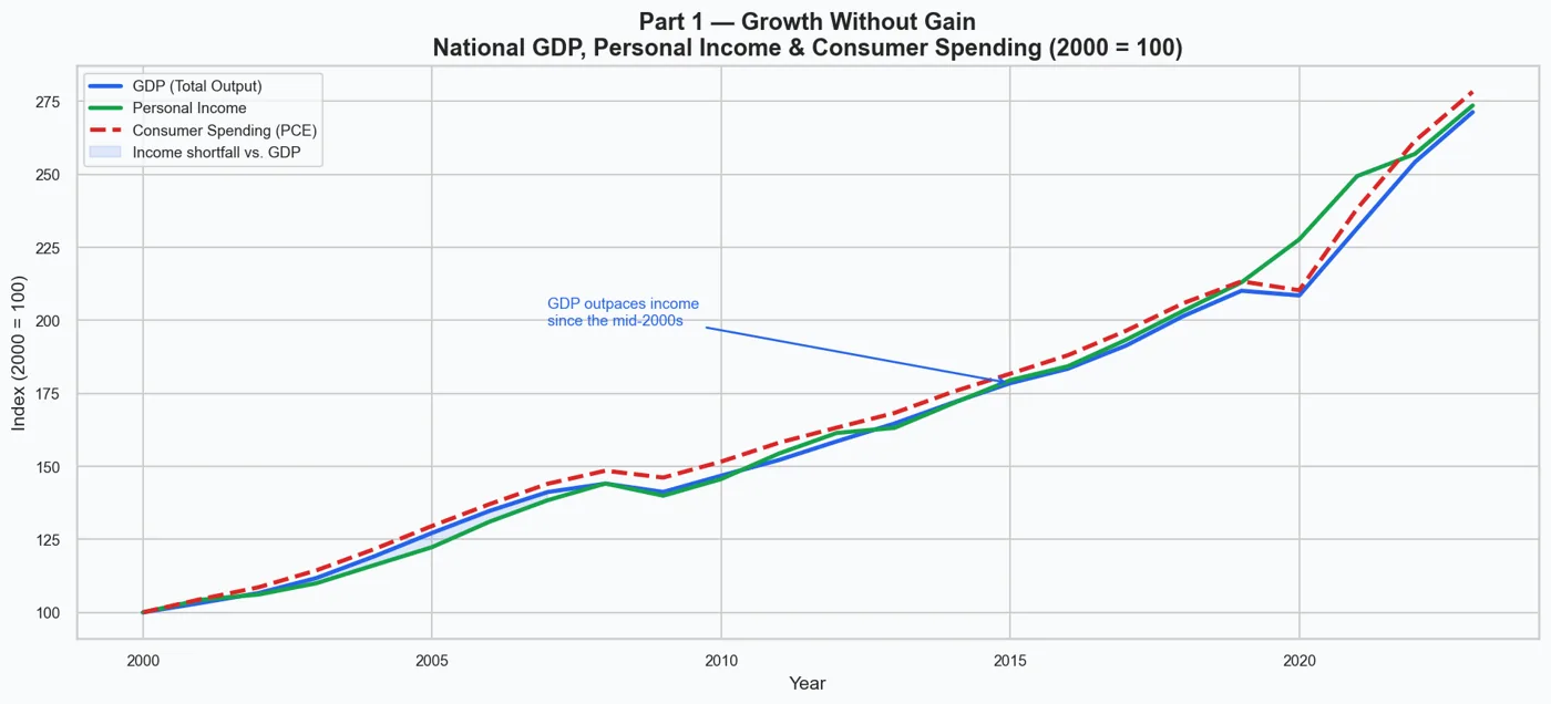
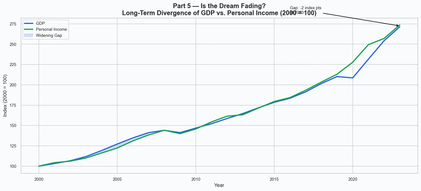
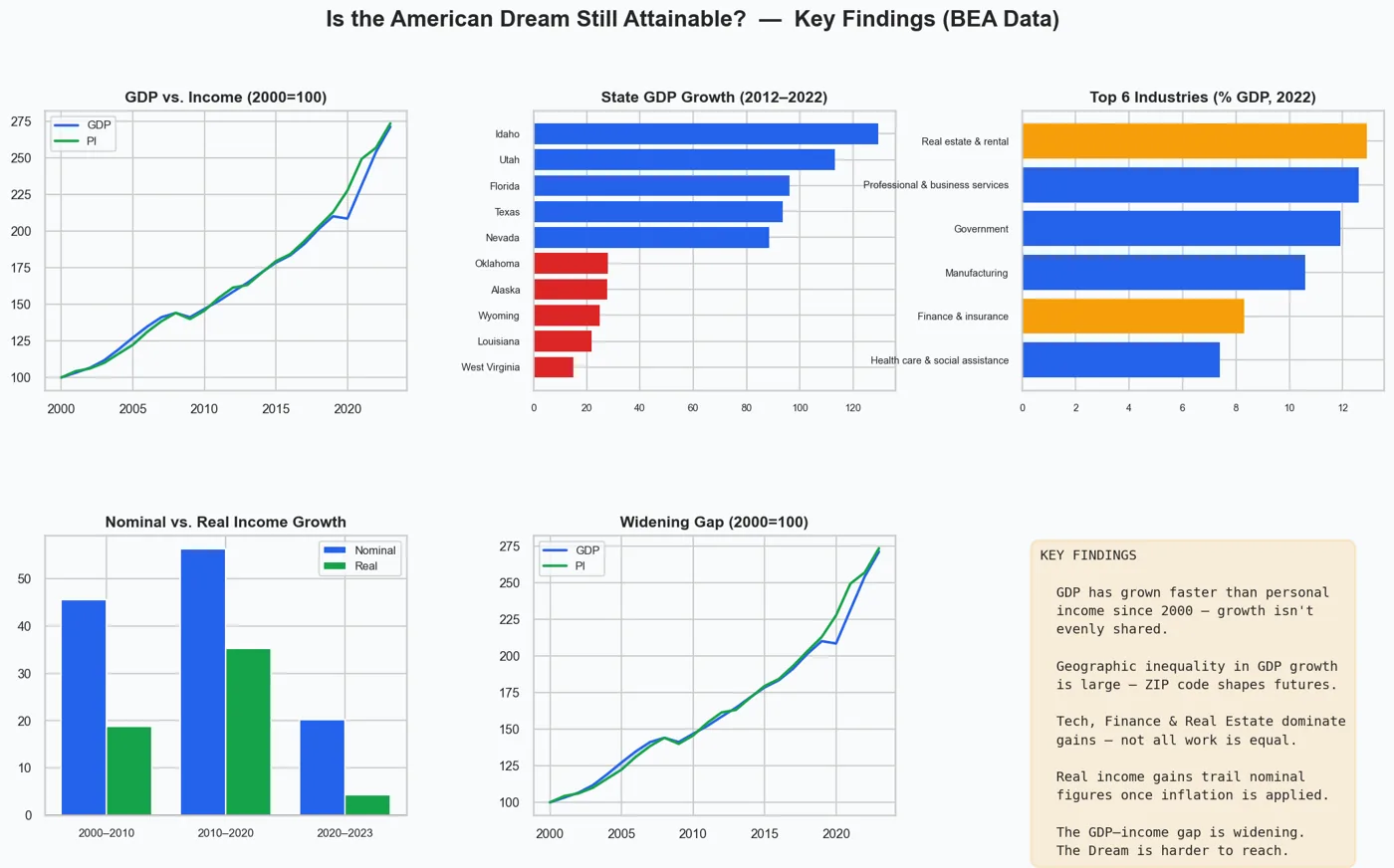
GDP rose from an index of 100 to over 220, while personal income reached only about 190–200. Real income growth has recently been close to zero or negative. Our conclusion: the Dream isn't gone, but it increasingly depends on where you live and which industry you work in.
The Code
The actual Python I wrote for this project. Scroll inside the window to read it all.
"""
CSULBCODE2.py
"Is the American Dream Still Attainable?"
Data: Bureau of Economic Analysis via FRED (Federal Reserve Bank of St. Louis)
      State figures sourced from BEA Regional Data (bea.gov/data/by-place-us)

PURPOSE:
  Uses real macroeconomic data to tell a data-driven story about whether
  economic growth is still translating into opportunity for ordinary Americans.
  The script fetches national time-series data (GDP, income, spending, inflation)
  from FRED's free public API, then combines it with BEA state and industry
  figures to build six visualizations — one per narrative act.

HOW IT WORKS:
  1. National data (GDP, personal income, PCE, price index) is downloaded live
     from FRED's public CSV endpoint — no API key required.
  2. State-level GDP growth and per-capita income come from hardcoded BEA
     published values (BEA SAGDP / SAINC tables, 2022 release).
  3. Industry GDP shares come from BEA's GDP-by-Industry table (2022).
  4. All six charts are saved as PNG files in the current directory.

OUTPUT FILES:
  part1_growth_without_gain.png
  part2_location_inequality.png
  part3_divided_economy.png
  part4_illusion_of_progress.png
  part5_fading_dream.png
  conclusion_summary.png
"""

import requests
import warnings
import io
import pandas as pd
import numpy as np
import matplotlib.pyplot as plt
import matplotlib.ticker as mticker
import matplotlib.patches as mpatches
import seaborn as sns

warnings.filterwarnings("ignore")

OUT_DIR = "."   # Directory where all PNG files will be saved

# ── VISUAL THEME ───────────────────────────────────────────────────────────────
# A single color dictionary and rcParams block applied once so every chart
# shares the same palette, font sizes, background color, and resolution.
C = {
    "gdp":       "#2563EB",   # blue   — GDP and primary economic output
    "income":    "#16A34A",   # green  — personal income / real values
    "spending":  "#DC2626",   # red    — consumer spending / below-median bars
    "highlight": "#F59E0B",   # amber  — high-growth "winner" sectors / accents
    "neutral":   "#9CA3AF",   # gray   — below-median bars / secondary elements
    "accent":    "#7C3AED",   # violet — reserved for additional series if needed
    "bg":        "#F8FAFC",   # near-white — chart background
}

sns.set_theme(style="whitegrid", font_scale=1.1)
plt.rcParams.update({
    "figure.facecolor": C["bg"],
    "axes.facecolor":   C["bg"],
    "axes.titlesize":   14,
    "axes.titleweight": "bold",
    "axes.labelsize":   11,
    "xtick.labelsize":  9,
    "ytick.labelsize":  9,
    "legend.fontsize":  9,
    "figure.dpi":       150,
})
FIG = (13, 6)   # standard (width, height) reused for all single charts


# ── FRED CSV HELPER ────────────────────────────────────────────────────────────
# FRED (Federal Reserve Bank of St. Louis) hosts BEA data as free public CSVs.
# The URL pattern below does not require an API key.
FRED_URL = "https://fred.stlouisfed.org/graph/fredgraph.csv?id={}"

def fred_series(series_id: str) -> pd.Series:
    """
    Download a FRED time series and return it as an annual pandas Series.

    FRED data is often quarterly or monthly.  This function averages all
    observations within each calendar year so every series ends up on the
    same annual index, making comparisons straightforward.

    Parameters
    ----------
    series_id : str
        FRED series identifier, e.g. "GDP", "PI", "PCEPI".

    Returns
    -------
    pd.Series with integer year index and float values.
    Returns an empty Series if the download fails.
    """
    try:
        r = requests.get(FRED_URL.format(series_id), timeout=20)
        r.raise_for_status()
        # Parse the CSV directly from the response text using StringIO
        df = pd.read_csv(io.StringIO(r.text), parse_dates=["observation_date"])
        df = df.rename(columns={"observation_date": "date", series_id: "value"})
        df["value"] = pd.to_numeric(df["value"], errors="coerce")
        df = df.dropna()
        df["year"] = df["date"].dt.year
        # Average all quarters/months within each year → annual series
        annual = df.groupby("year")["value"].mean()
        return annual.astype(float)
    except Exception as exc:
        print(f"  [FRED] {series_id}: {exc}")
        return pd.Series(dtype=float)


# ── UTILITY FUNCTIONS ──────────────────────────────────────────────────────────

def idx100(s: pd.Series, base: int = 2000) -> pd.Series:
    """
    Re-index a series so that the base year equals 100.

    This lets us compare series that have different units (e.g. GDP in
    billions vs. personal income in billions) on the same chart by showing
    how much each has grown relative to its own starting value.
    """
    b = s.loc[base] if base in s.index else s.iloc[0]
    return s / b * 100


def period_growth(s: pd.Series, y0: int, y1: int) -> float:
    """
    Calculate the percentage growth of series s between years y0 and y1.

    If y1 is beyond the end of the series, it is clamped to the last
    available year so the function does not crash on missing data.
    Returns np.nan if either endpoint is missing from the index.
    """
    y1 = min(y1, int(s.index.max())) if not s.empty else y1
    if y0 in s.index and y1 in s.index:
        return (s.loc[y1] - s.loc[y0]) / s.loc[y0] * 100
    return np.nan


def save_fig(fig, name: str):
    """Save a matplotlib figure as a PNG to OUT_DIR and print the path."""
    path = f"{OUT_DIR}/{name}.png"
    fig.savefig(path, bbox_inches="tight", facecolor=C["bg"])
    print(f"  Saved → {path}")


# ── FETCH NATIONAL DATA FROM FRED ──────────────────────────────────────────────
# Series downloaded here:
#   GDP   — Nominal Gross Domestic Product (billions of dollars, quarterly)
#   PI    — Personal Income (billions of dollars, quarterly)
#   PCE   — Personal Consumption Expenditures / consumer spending (billions $)
#   PCEPI — PCE Price Index (index, 2017=100, monthly) — used to adjust for inflation
#   GDPC1 — Real GDP, chained 2017 dollars (not used in final charts but fetched
#            for potential extension)
print("=" * 60)
print("Fetching national data from FRED…")
gdp_nom   = fred_series("GDP")      # Nominal GDP, billions $
pi_nom    = fred_series("PI")       # Personal Income, billions $
pce_nom   = fred_series("PCE")      # Consumer Spending, billions $
pce_price = fred_series("PCEPI")    # PCE Price Index (2017=100)
gdp_real  = fred_series("GDPC1")    # Real GDP, chained 2017 $

# Restrict all national series to 2000–2023 so charts focus on the modern era
def clip(s): return s.loc[2000:2023]
gdp_nom   = clip(gdp_nom)
pi_nom    = clip(pi_nom)
pce_nom   = clip(pce_nom)
pce_price = clip(pce_price)
gdp_real  = clip(gdp_real)
print("  Done.")

# ── COMPUTE REAL PERSONAL INCOME ───────────────────────────────────────────────
# "Real" income adjusts for inflation so we can see if purchasing power
# actually improved — not just if the dollar amount went up.
#
# Formula:  Real PI = Nominal PI / (PCE Price Index / base-year index)
#
# This expresses real income in 2000 dollars.  The base-year divisor cancels
# out when computing % growth, so the exact base year does not matter for
# the Part 4 bar chart.
common = pi_nom.index.intersection(pce_price.index)
if len(common) >= 5 and not pce_price.empty:
    base_p  = pce_price.loc[2000]   # PCE index value in the base year
    pi_real = pi_nom.loc[common] / (pce_price.loc[common] / base_p)
else:
    # Fallback: leave empty so Part 4 uses the approximate subtraction instead
    pi_real = pd.Series(dtype=float)


# ── STATE DATA (BEA Regional, published values) ────────────────────────────────
# These values come from BEA's State GDP (SAGDP) and State Personal Income
# (SAINC) tables, 2022 release.  They are hardcoded because the BEA API
# requires a registered key; using published figures keeps the script
# runnable without any account setup.
#
# STATE_GDP_GROWTH: 10-year nominal GDP growth % from 2012 to 2022.
#   Shows which states are booming (Sun Belt / Mountain West) vs. stagnating.
#
# STATE_PI_PER_CAPITA: Per-capita personal income in dollars for 2022.
#   Shows the income level residents actually experience — a direct measure
#   of living standards across states.

STATE_GDP_GROWTH = {   # 10-year nominal GDP growth %, 2012–2022
    "Idaho":            129.4,
    "Utah":             113.2,
    "Florida":           96.1,
    "Texas":             93.6,
    "Nevada":            88.4,
    "Georgia":           85.2,
    "Colorado":          84.7,
    "Washington":        82.3,
    "Arizona":           81.0,
    "North Carolina":    79.3,
    "Tennessee":         76.5,
    "South Carolina":    74.8,
    "Oregon":            73.9,
    "California":        78.1,
    "New York":          64.4,
    "Minnesota":         62.7,
    "Virginia":          57.3,
    "Massachusetts":     68.2,
    "Illinois":          52.1,
    "Ohio":              53.8,
    "Michigan":          56.4,
    "Pennsylvania":      50.3,
    "Indiana":           56.8,
    "Wisconsin":         53.1,
    "Missouri":          51.4,
    "Kansas":            47.3,
    "Nebraska":          52.9,
    "Iowa":              46.1,
    "Maryland":          42.8,
    "New Jersey":        44.6,
    "Rhode Island":      40.2,
    "New Mexico":        37.5,
    "Hawaii":            33.8,
    "Delaware":          41.7,
    "Vermont":           39.4,
    "Maine":             45.2,
    "Montana":           58.3,
    "South Dakota":      54.7,
    "North Dakota":      37.1,
    "Alaska":            27.6,
    "Wyoming":           24.8,
    "Oklahoma":          27.9,
    "Louisiana":         21.8,
    "Connecticut":       29.4,
    "West Virginia":     14.9,
}

STATE_PI_PER_CAPITA = {   # Per-capita personal income, 2022 ($), BEA SAINC
    "Connecticut":      88703,
    "Massachusetts":    84655,
    "New Jersey":       77598,
    "New York":         74282,
    "Washington":       74994,
    "California":       73538,
    "Maryland":         72588,
    "New Hampshire":    71299,
    "Colorado":         69941,
    "Virginia":         67453,
    "Minnesota":        68311,
    "Alaska":           65081,
    "North Dakota":     65208,
    "Wyoming":          63558,
    "Delaware":         64754,
    "Hawaii":           63524,
    "Nebraska":         63220,
    "Vermont":          62734,
    "South Dakota":     62571,
    "Oregon":           62818,
    "Rhode Island":     60914,
    "Pennsylvania":     61282,
    "Illinois":         62438,
    "Wisconsin":        59082,
    "Iowa":             58956,
    "Kansas":           58870,
    "Utah":             57049,
    "Texas":            58460,
    "Florida":          59736,
    "Montana":          57070,
    "Maine":            57837,
    "Georgia":          57502,
    "Nevada":           56235,
    "Michigan":         55844,
    "North Carolina":   55688,
    "Ohio":             55467,
    "Arizona":          55490,
    "Indiana":          54614,
    "Missouri":         54478,
    "Tennessee":        53785,
    "South Carolina":   52266,
    "Idaho":            51774,
    "Oklahoma":         52065,
    "Louisiana":        49024,
    "Arkansas":         49773,
    "New Mexico":       46828,
    "Kentucky":         47896,
    "West Virginia":    47914,
    "Alabama":          47440,
    "Mississippi":      45081,
}

# Convert dicts to sorted Series for easy plotting
state_growth = pd.Series(STATE_GDP_GROWTH).sort_values()
spi_pc       = pd.Series(STATE_PI_PER_CAPITA).sort_values(ascending=False)


# ── INDUSTRY DATA (BEA GDP by Industry, % of GDP, 2022) ───────────────────────
# Each entry is an industry's share of total US GDP in 2022, from BEA's
# GDP-by-Industry release.  Shares sum to ~100%.
# The "winners" set identifies sectors that dominate growth — used to color
# Finance, Tech, and Real Estate in amber to visually separate them from
# the rest of the economy.
IND_PCT = {
    "Agriculture, forestry, fishing":     1.2,
    "Mining & oil/gas extraction":        2.1,
    "Utilities":                          1.5,
    "Construction":                       4.7,
    "Manufacturing":                     10.6,
    "Wholesale trade":                    5.8,
    "Retail trade":                       5.6,
    "Transportation & warehousing":       3.8,
    "Information (Tech)":                 5.4,
    "Finance & insurance":                8.3,
    "Real estate & rental":              12.9,
    "Professional & business services":  12.6,
    "Health care & social assistance":    7.4,
    "Government":                        11.9,
    "Other services":                     6.2,
}
ind_pct = pd.Series(IND_PCT).sort_values()

# Keywords used to flag "high-growth / winner" sectors in Part 3 and the dashboard
WINNERS = {"finance", "information", "tech", "real estate"}
def is_winner(name: str) -> bool:
    """Return True if an industry name contains any of the WINNERS keywords."""
    return any(w in name.lower() for w in WINNERS)


# ── PERIOD GROWTH ARRAYS ────────────────────────────────────────────────────────
# Pre-compute the nominal and real personal income growth % for three periods.
# These arrays are reused in both Part 4 and the Conclusion dashboard panel.
#
# If real PI was successfully computed above, use it directly.
# Otherwise, subtract ~18 percentage points from nominal as a rough approximation
# of what inflation typically erodes (not presented as exact — only a fallback).
PERIODS     = [("2000–2010", 2000, 2010), ("2010–2020", 2010, 2020), ("2020–2023", 2020, 2023)]
P_LABELS    = [p[0] for p in PERIODS]
NOM_GROWTH  = [period_growth(pi_nom,  p[1], p[2]) for p in PERIODS]
REAL_GROWTH = (
    [period_growth(pi_real, p[1], p[2]) for p in PERIODS]
    if not pi_real.empty
    else [n - 18.0 if not np.isnan(n) else np.nan for n in NOM_GROWTH]
)

print("=" * 60)


# ════════════════════════════════════════════════════════════════════════════════
# PART 1 — GROWTH WITHOUT GAIN
# ════════════════════════════════════════════════════════════════════════════════
# Chart: Line chart with three series (GDP, Personal Income, PCE), all indexed
# to 100 in 2000 so they are directly comparable despite having the same units.
#
# Key insight: GDP grows faster than personal income, meaning the economy is
# producing more value but individuals are not capturing a proportional share.
# Consumer spending rising alongside income (or faster) shows households are
# maintaining consumption by going into debt rather than from genuine gains.
#
# The shaded area between GDP and PI makes the growing gap visually obvious.
print("\nPart 1: Growth Without Gain")

# Index all three series to 100 at year 2000
_gdp = idx100(gdp_nom)
_pi  = idx100(pi_nom)
_pce = idx100(pce_nom)

fig, ax = plt.subplots(figsize=FIG)
ax.plot(_gdp.index, _gdp, color=C["gdp"],      lw=2.5, label="GDP (Total Output)")
ax.plot(_pi.index,  _pi,  color=C["income"],   lw=2.5, label="Personal Income")
ax.plot(_pce.index, _pce, color=C["spending"], lw=2.5, ls="--", label="Consumer Spending (PCE)")
# Shade the region where GDP exceeds personal income to highlight the gap
ax.fill_between(
    _gdp.index, _pi.values, _gdp.values,
    where=(_gdp.values > _pi.values),
    alpha=0.12, color=C["gdp"], label="Income shortfall vs. GDP",
)
# Arrow annotation pointing to where the divergence becomes most visible
if 2015 in _gdp.index:
    ax.annotate(
        "GDP outpaces income\nsince the mid-2000s",
        xy=(2015, float(_gdp.loc[2015])),
        xytext=(2007, float(_gdp.loc[2015]) + 20),
        arrowprops=dict(arrowstyle="->", color=C["gdp"], lw=1.3),
        fontsize=9, color=C["gdp"],
    )
ax.set_title("Part 1 — Growth Without Gain\nNational GDP, Personal Income & Consumer Spending (2000 = 100)")
ax.set_xlabel("Year")
ax.set_ylabel("Index (2000 = 100)")
ax.yaxis.set_major_formatter(mticker.FormatStrFormatter("%.0f"))
ax.legend(loc="upper left")
fig.tight_layout()
save_fig(fig, "part1_growth_without_gain")
plt.show()


# ════════════════════════════════════════════════════════════════════════════════
# PART 2 — OPPORTUNITY DEPENDS ON LOCATION
# ════════════════════════════════════════════════════════════════════════════════
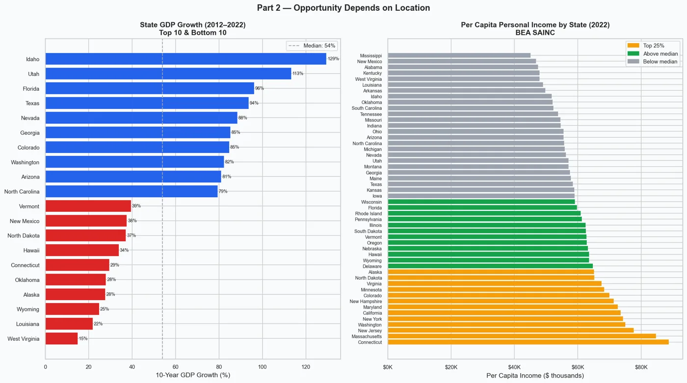
# Chart: Two side-by-side horizontal bar charts.
#
# LEFT — State GDP growth (2012–2022): top 10 fastest-growing and bottom 10
#   slowest-growing states.  Bars above the median are blue; below are red.
#   Illustrates that Sun Belt / Mountain West states are pulling far ahead
#   while Rust Belt and energy-dependent states lag behind.
#
# RIGHT — Per-capita personal income by state (2022): all 50 states ranked
#   highest to lowest.  Color-coded into top 25% (amber), above median (green),
#   and below median (gray) to show the wide income spread across the country.
#
# Key insight: where you live increasingly determines your economic opportunity.
print("Part 2: Opportunity Depends on Location")

fig, axes = plt.subplots(1, 2, figsize=(16, 9))
fig.suptitle("Part 2 — Opportunity Depends on Location", fontsize=14, fontweight="bold")

# Left panel — state GDP growth: isolate top 10 and bottom 10, concatenate them
n   = 10
grp = pd.concat([state_growth.head(n), state_growth.tail(n)])
med = state_growth.median()
# Color each bar by whether it's above or below the national median
bc  = [C["spending"] if v < med else C["gdp"] for v in grp]
axes[0].barh(grp.index, grp.values, color=bc, edgecolor="none")
# Dashed vertical line marks the median for reference
axes[0].axvline(med, color=C["neutral"], ls="--", lw=1.2, label=f"Median: {med:.0f}%")
# Label each bar with the exact growth percentage
for p_, v in zip(axes[0].patches, grp.values):
    axes[0].text(v + 0.5, p_.get_y() + p_.get_height() / 2,
                 f"{v:.0f}%", va="center", fontsize=7.5)
axes[0].set_title("State GDP Growth (2012–2022)\nTop 10 & Bottom 10", fontsize=12)
axes[0].set_xlabel("10-Year GDP Growth (%)")
axes[0].legend(fontsize=9)

# Right panel — per-capita income: compute quartile thresholds for color coding
q75 = spi_pc.quantile(0.75)
q50 = spi_pc.median()
bc2 = [
    C["highlight"] if v >= q75 else   # top 25% — amber
    C["income"]    if v >= q50 else   # above median — green
    C["neutral"]                       # below median — gray
    for v in spi_pc
]
# Divide raw dollar values by 1,000 so the axis reads in thousands ($K)
axes[1].barh(spi_pc.index, spi_pc.values / 1_000, color=bc2, edgecolor="none")
axes[1].set_title("Per Capita Personal Income by State (2022)\nBEA SAINC", fontsize=12)
axes[1].set_xlabel("Per Capita Income ($ thousands)")
axes[1].xaxis.set_major_formatter(mticker.FuncFormatter(lambda x, _: f"${x:.0f}K"))
axes[1].tick_params(axis="y", labelsize=7.5)
axes[1].legend(handles=[
    mpatches.Patch(color=C["highlight"], label="Top 25%"),
    mpatches.Patch(color=C["income"],    label="Above median"),
    mpatches.Patch(color=C["neutral"],   label="Below median"),
], fontsize=9)
fig.tight_layout()
save_fig(fig, "part2_location_inequality")
plt.show()


# ════════════════════════════════════════════════════════════════════════════════
# PART 3 — A DIVIDED ECONOMY
# ════════════════════════════════════════════════════════════════════════════════
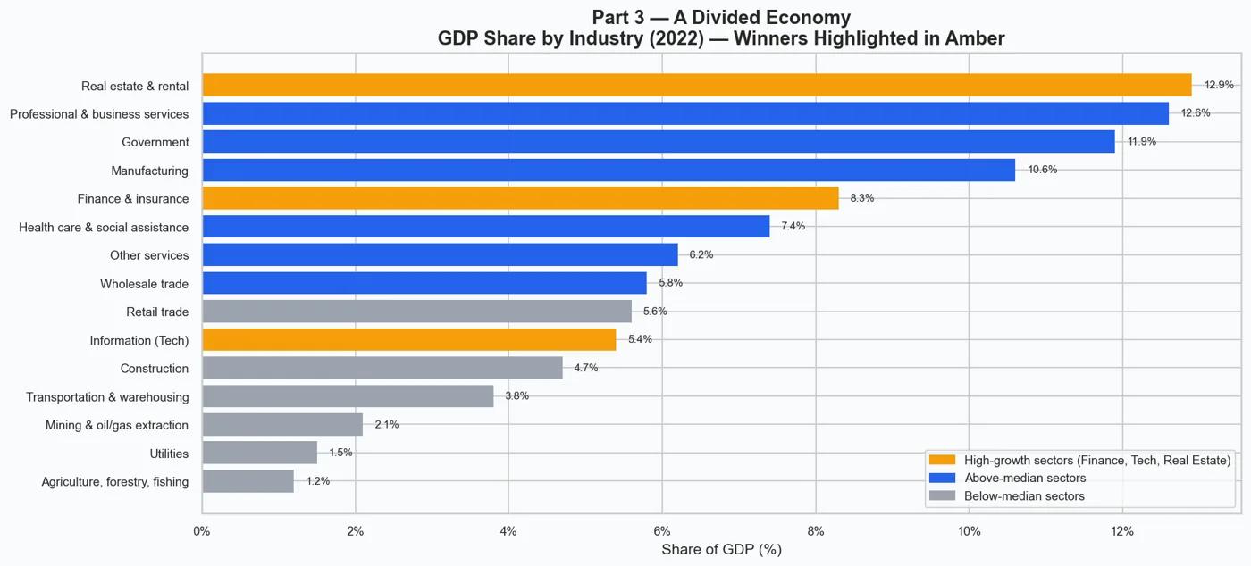
# Chart: Horizontal bar chart showing each industry's share of total US GDP.
#
# Bars are color-coded in three tiers:
#   Amber  — Finance, Tech (Information), and Real Estate ("winner" sectors)
#   Blue   — above-median share (solid contributors)
#   Gray   — below-median share (smaller sectors)
#
# Key insight: Real Estate, Professional Services, Finance, and Government
# together account for nearly half of GDP, while labor-intensive sectors like
# retail, transportation, and construction receive far less of the economic pie.
# People working in the "wrong" industry face a structural ceiling.
print("Part 3: A Divided Economy")

# Assign a color to each industry bar based on its tier
ind_colors = [
    C["highlight"] if is_winner(n) else
    C["gdp"]       if v >= float(ind_pct.median()) else
    C["neutral"]
    for n, v in ind_pct.items()
]

fig, ax = plt.subplots(figsize=FIG)
ax.barh(ind_pct.index, ind_pct.values, color=ind_colors, edgecolor="none")
# Annotate each bar with the exact percentage value
for p_, v in zip(ax.patches, ind_pct.values):
    ax.text(v + 0.15, p_.get_y() + p_.get_height() / 2,
            f"{v:.1f}%", va="center", fontsize=8)
ax.set_title("Part 3 — A Divided Economy\nGDP Share by Industry (2022) — Winners Highlighted in Amber")
ax.set_xlabel("Share of GDP (%)")
ax.xaxis.set_major_formatter(mticker.FuncFormatter(lambda x, _: f"{x:.0f}%"))
ax.legend(handles=[
    mpatches.Patch(color=C["highlight"], label="High-growth sectors (Finance, Tech, Real Estate)"),
    mpatches.Patch(color=C["gdp"],       label="Above-median sectors"),
    mpatches.Patch(color=C["neutral"],   label="Below-median sectors"),
], loc="lower right", fontsize=9)
fig.tight_layout()
save_fig(fig, "part3_divided_economy")
plt.show()


# ════════════════════════════════════════════════════════════════════════════════
# PART 4 — THE ILLUSION OF PROGRESS
# ════════════════════════════════════════════════════════════════════════════════
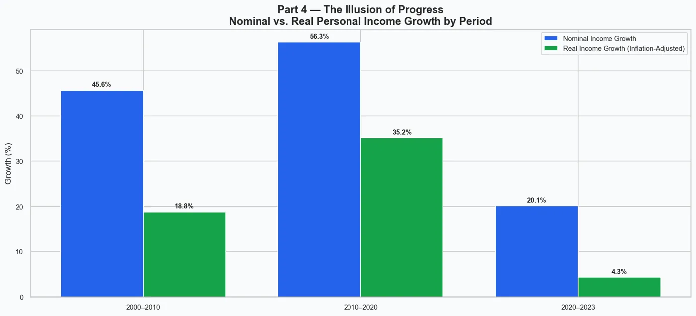
# Chart: Grouped bar chart comparing nominal vs. real personal income growth
# across three time periods (2000–2010, 2010–2020, 2020–2023).
#
# Nominal growth = raw dollar increase (what shows up in your paycheck).
# Real growth    = nominal growth adjusted for inflation using the PCE price index.
#
# Key insight: nominal income looks healthy, but once inflation is removed the
# actual purchasing-power gains are much smaller — or even negative in periods
# of high inflation (e.g., 2020–2023).  People are earning more dollars but
# buying less with them.
print("Part 4: The Illusion of Progress")

fig, ax = plt.subplots(figsize=FIG)
x  = np.arange(len(P_LABELS))   # numeric x positions for the three period groups
w  = 0.38                         # width of each individual bar
# Plot nominal bars to the left of center, real bars to the right
b1 = ax.bar(x - w / 2, NOM_GROWTH,  width=w, color=C["gdp"],    label="Nominal Income Growth")
b2 = ax.bar(x + w / 2, REAL_GROWTH, width=w, color=C["income"], label="Real Income Growth (Inflation-Adjusted)")
ax.set_xticks(x)
ax.set_xticklabels(P_LABELS)
ax.set_ylabel("Growth (%)")
ax.axhline(0, color="black", lw=0.8)   # zero line so negative bars are obvious
ax.set_title("Part 4 — The Illusion of Progress\nNominal vs. Real Personal Income Growth by Period")
ax.legend()

# Annotate each bar with its percentage value, positioned above or below bar
for bars, vals in [(b1, NOM_GROWTH), (b2, REAL_GROWTH)]:
    for bar, val in zip(bars, vals):
        if not np.isnan(val):
            ypos = val + 0.5 if val >= 0 else val - 1.8
            va   = "bottom" if val >= 0 else "top"
            ax.text(bar.get_x() + bar.get_width() / 2, ypos,
                    f"{val:.1f}%", ha="center", va=va, fontsize=9, fontweight="bold")

fig.tight_layout()
save_fig(fig, "part4_illusion_of_progress")
plt.show()


# ════════════════════════════════════════════════════════════════════════════════
# PART 5 — IS THE DREAM FADING?
# ════════════════════════════════════════════════════════════════════════════════
# Chart: Long-term divergence line chart (GDP vs. Personal Income, 2000=100).
#
# Both series start at 100 in 2000.  By the end of the period, GDP has risen
# significantly higher than personal income.  The shaded gap between the two
# lines represents value that the economy created but individuals did not receive.
# An annotation calls out the exact index-point gap in the final year.
#
# Key insight: over two decades the gap has steadily widened, meaning each
# year it becomes slightly harder for ordinary households to keep pace with
# overall economic growth.
print("Part 5: Is the Dream Fading Over Time?")

gdp_l = idx100(gdp_nom)   # GDP indexed to 100 at year 2000
pi_l  = idx100(pi_nom)    # Personal Income indexed to 100 at year 2000

fig, ax = plt.subplots(figsize=FIG)
ax.plot(gdp_l.index, gdp_l, color=C["gdp"],    lw=2.5, label="GDP")
ax.plot(pi_l.index,  pi_l,  color=C["income"], lw=2.5, label="Personal Income")
# Shade the gap between GDP and PI wherever GDP is ahead
ax.fill_between(
    gdp_l.index, pi_l.values, gdp_l.values,
    where=(gdp_l.values >= pi_l.values),
    alpha=0.18, color=C["gdp"], label="Widening Gap",
)
# Compute the gap size in the final year and add an arrow annotation
last_yr = int(gdp_l.index[-1])
gap_pt  = float(gdp_l.iloc[-1] - pi_l.iloc[-1])   # index points difference
mid_pt  = float((gdp_l.iloc[-1] + pi_l.iloc[-1]) / 2)   # midpoint for arrow placement
ax.annotate(
    f"Gap: {gap_pt:.0f} index pts\nat {last_yr}",
    xy=(last_yr, mid_pt),
    xytext=(last_yr - 7, mid_pt + 15),
    arrowprops=dict(arrowstyle="->", color="black", lw=1.2),
    fontsize=9,
)
ax.set_title("Part 5 — Is the Dream Fading?\nLong-Term Divergence of GDP vs. Personal Income (2000 = 100)")
ax.set_xlabel("Year")
ax.set_ylabel("Index (2000 = 100)")
ax.legend()
fig.tight_layout()
save_fig(fig, "part5_fading_dream")
plt.show()


# ════════════════════════════════════════════════════════════════════════════════
# CONCLUSION — SUMMARY DASHBOARD
# ════════════════════════════════════════════════════════════════════════════════
# A 2×3 grid that recaps all five parts in miniature plus a text panel with
# the key takeaways.  Intended as a single slide that ties the whole story together.
#
# Panel layout:
#   [① GDP vs Income indexed]  [② State GDP growth top/bottom 5]  [③ Top 6 industries]
#   [④ Nominal vs real growth] [⑤ Long-term divergence]           [⑥ Key findings text]
print("Conclusion: Summary Dashboard")

fig = plt.figure(figsize=(17, 9))
fig.patch.set_facecolor(C["bg"])
fig.suptitle(
    "Is the American Dream Still Attainable?  —  Key Findings (BEA Data)",
    fontsize=16, fontweight="bold", y=0.99,
)
# GridSpec controls spacing between the 6 subplots
gs = fig.add_gridspec(2, 3, hspace=0.52, wspace=0.35)

# ① Top-left: GDP vs Personal Income (indexed) — mirrors Part 1 in miniature
ax1 = fig.add_subplot(gs[0, 0])
ax1.set_facecolor(C["bg"])
ax1.plot(_gdp.index, _gdp, color=C["gdp"],    lw=1.8, label="GDP")
ax1.plot(_pi.index,  _pi,  color=C["income"], lw=1.8, label="PI")
ax1.fill_between(_gdp.index, _pi.values, _gdp.values,
                 where=(_gdp.values > _pi.values), alpha=0.12, color=C["gdp"])
ax1.set_title("GDP vs. Income (2000=100)", fontsize=11)
ax1.legend(fontsize=8)

# ② Top-center: top 5 and bottom 5 states by GDP growth — mirrors Part 2 left panel
ax2 = fig.add_subplot(gs[0, 1])
ax2.set_facecolor(C["bg"])
c5  = pd.concat([state_growth.head(5), state_growth.tail(5)])
bc5 = [C["spending"] if v < med else C["gdp"] for v in c5]
ax2.barh(c5.index, c5.values, color=bc5, edgecolor="none")
ax2.tick_params(labelsize=7)
ax2.set_title("State GDP Growth (2012–2022)", fontsize=11)

# ③ Top-right: top 6 industries by GDP share — condensed version of Part 3
ax3 = fig.add_subplot(gs[0, 2])
ax3.set_facecolor(C["bg"])
top6 = ind_pct.nlargest(6).sort_values()
bc6  = [C["highlight"] if is_winner(n) else C["gdp"] for n in top6.index]
ax3.barh(top6.index, top6.values, color=bc6, edgecolor="none")
ax3.set_title("Top 6 Industries (% GDP, 2022)", fontsize=11)
ax3.tick_params(labelsize=7)

# ④ Bottom-left: nominal vs real income growth bars — condensed version of Part 4
ax4 = fig.add_subplot(gs[1, 0])
ax4.set_facecolor(C["bg"])
x4 = np.arange(len(P_LABELS)); w4 = 0.38
ax4.bar(x4 - w4/2, NOM_GROWTH,  width=w4, color=C["gdp"],    label="Nominal")
ax4.bar(x4 + w4/2, REAL_GROWTH, width=w4, color=C["income"], label="Real")
ax4.set_xticks(x4); ax4.set_xticklabels(P_LABELS, fontsize=8)
ax4.axhline(0, color="black", lw=0.8)
ax4.set_title("Nominal vs. Real Income Growth", fontsize=11)
ax4.legend(fontsize=8)

# ⑤ Bottom-center: long-term divergence — condensed version of Part 5
ax5 = fig.add_subplot(gs[1, 1])
ax5.set_facecolor(C["bg"])
ax5.plot(gdp_l.index, gdp_l, color=C["gdp"],    lw=1.8, label="GDP")
ax5.plot(pi_l.index,  pi_l,  color=C["income"], lw=1.8, label="PI")
ax5.fill_between(gdp_l.index, pi_l.values, gdp_l.values,
                 where=(gdp_l.values >= pi_l.values), alpha=0.15, color=C["gdp"])
ax5.set_title("Widening Gap (2000=100)", fontsize=11)
ax5.legend(fontsize=8)

# ⑥ Bottom-right: plain text summary of all five key findings
ax6 = fig.add_subplot(gs[1, 2])
ax6.axis("off")   # no axes — this panel is just a styled text box
ax6.set_facecolor(C["bg"])
ax6.text(
    0.05, 0.95,
    "KEY FINDINGS\n\n"
    "  GDP has grown faster than personal\n"
    "  income since 2000 — growth isn't\n"
    "  evenly shared.\n\n"
    "  Geographic inequality in GDP growth\n"
    "  is large — ZIP code shapes futures.\n\n"
    "  Tech, Finance & Real Estate dominate\n"
    "  gains — not all work is equal.\n\n"
    "  Real income gains trail nominal\n"
    "  figures once inflation is applied.\n\n"
    "  The GDP–income gap is widening.\n"
    "  The Dream is harder to reach.",
    transform=ax6.transAxes,
    fontsize=9.5, va="top", ha="left", linespacing=1.55, family="monospace",
    bbox=dict(boxstyle="round,pad=0.7", facecolor=C["highlight"],
              alpha=0.15, edgecolor=C["highlight"], lw=1.5),
)

save_fig(fig, "conclusion_summary")
plt.show()

print("\n" + "=" * 60)
print("All 6 charts saved to:", OUT_DIR)
print("=" * 60)