Overview
For this data visualization final, I explored a credit-approval dataset through a dozen chart types in Python. The course also covered dashboards in Tableau.
Key results
12analysis questions, each answered with the best-fitting chart type
Age ↔ Debtthe strongest relationship among age, income and debt
The question
Which applicant traits (income, debt, years employed, marital status) relate to credit approval, and how do you show each relationship most clearly?
What I did
- Joint plots and correlation views for age, income and debt
- KDE and box plots to compare distributions across groups
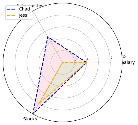
- Radar charts to compare normalized income sources
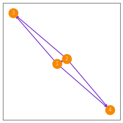
- A network graph showing how communication flows in a team
What I found
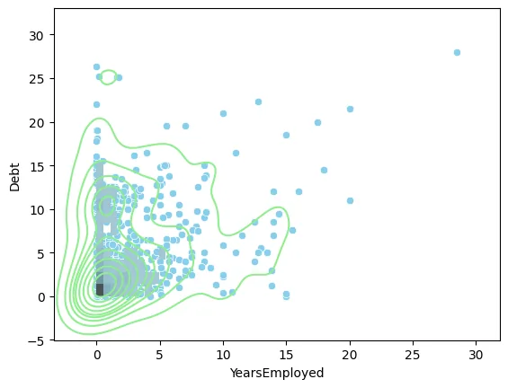
Applicants with higher income and lower debt were more likely to be approved, and people with more years of employment tended to carry less debt. The bigger lesson was matching the chart to the question.
The Code
The actual Python I wrote for this project. Scroll inside the window to read it all.
import seaborn as sns
import matplotlib.pyplot as plt
import numpy as np
import pandas as pd

df = pd.read_csv('clean_dataset.csv')
df.head()

#1
sns.catplot(data=df, y='Debt', x='Citizen', kind= 'box', hue= 'Citizen')
plt.xticks(rotation=20)
plt.show()

#On average, people who are born in the country tend
#have more debt than those who are in the coutnry by other means, and temporary

#2
#age and debt corr
plt.figure(figsize=(8,4))
sns.jointplot(data=df, x='Age', y='Debt', kind='reg')
plt.show()

#age and income corr
plt.figure(figsize=(8,4))
sns.jointplot(data=df, x='Age', y='Income', kind='reg')
plt.show()

#debt and income corr
plt.figure(figsize=(8,4))
sns.jointplot(data=df, x='Debt', y='Income', kind='reg')
plt.show()

#We found that the strongesrt correlation is between Age and debr dramatically more
#than the correlations between debt and income, and lastly by age and income

#3

Industry_count= df['Industry'].value_counts()
Industry_count

Industry_pie= df['Industry'].value_counts().index.tolist()
Industry_pie

plt.figure(figsize=(6,6))
plt.pie(Industry_count, labels=Industry_pie, autopct= '%1.2f%%')
plt.show()

#By looking at the pie chart above, we foudn that the only industry group compromising at leats 20%
#of the overall customer population is Energy.

#4
plt.figure(figsize=(6,5))
sns.scatterplot(data=df, y='Income', x='Debt', hue='Approved', marker='x', s=50)
plt.show()

#Based on the scatter plot above on Debt and Income, we found that a person will usually have
#a higher chance of getting approved for credit if they have a higher income and less debt

#5
plt.figure(figsize=(10,5))
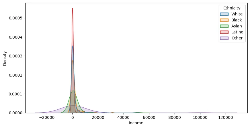
sns.kdeplot(data=df, x='Income', hue='Ethnicity', fill=True,
            alpha=0.2, linewidth=1, linestyle='-', common_norm=False)
plt.show()

#Based on the kde plot above, we can see that the ethnicity with the smallest income gap
#is Latino and majority of their distrubution having about 0 income compared to the other ethnicities.

#6
sns.catplot(data=df, y='Debt', x='Married', kind= 'box', hue= 'Married')
plt.show()

#Based on the box plot above we found that on average, married people are more
#likely to have debt. Even with single people having more debt outliers

#7
#plt.figure(figsize=(5,3))
#sns.scatterplot(data=df, x='YearsEmployed', y='Debt')
#plt.show()

sns.scatterplot(data=df, x='YearsEmployed', y='Debt', color='skyblue')
sns.histplot(data=df, x='YearsEmployed', y='Debt', color ='lightblue', pthresh=0.2)
sns.kdeplot(data=df, x='YearsEmployed', y='Debt', color='lightgreen')
plt.show()

#Based off the stacked plot above (scatter, hist, kde), we foudn that people
#who have worked longer tend to have less debt than than those who just started working

#8
sns.catplot(data=df, x= 'Ethnicity', y='Debt', kind= 'box',
            hue= 'Married')
plt.show()

#Based off the box plots above, by looking only at the married couples by ethnicity
#white couples tend to have the lowest debt on average

#9
#define Incomes
attributes= ['Salary', 'Side Hustles', 'Stocks',]
values_chad= [4, 5, 10]
values_chad= values_chad +[4]
values_chad

values_jess= [4, 0, 8]
values_jess= values_jess + [4]
values_jess

#define angles
angles = np.linspace(0, 2*np.pi, 3, endpoint=False).tolist()
angles = angles+ [0]
angles

#initialize the radar chart
plt.figure(figsize=(5,5))
ax= plt.subplot(polar=True)
#add attributes/features
plt.xticks(angles[:-1], attributes)
ax.set_rlabel_position(4)
plt.yticks([2,4,6,8,10], color="blue", alpha=0.8, size=7)
plt.ylim(0,10)
#add Chad info
ax.plot(angles, values_chad, label='Chad',color='blue',linewidth=2, linestyle='--')
ax.fill(angles, values_chad, alpha=0.4, facecolor='pink')
#add Jess info
ax.plot(angles, values_jess, label='Jess',linewidth=2, color='orange', linestyle='--')
ax.fill(angles, values_jess, alpha=0.2, facecolor='lightgreen')
plt.legend(loc='upper left')
plt.show()

#the visualization above shows the comparison between Chad and jess's sources of income after being normalized.
#they show that Chad over all makes more money

#10
def func_(x):
  outcome= 2000 +x**2
  return outcome

x = np.linspace(0,12, 100) + 6
y = func_(x)

plt.figure(figsize=(4, 4))
plt.plot(x, y, color='indigo', linestyle='--', linewidth=3)
plt.axvline(x=6, color= 'red', linestyle= '--', linewidth=1.3)
plt.grid()
plt.show()

#the graph above shows the savings increasing after month 6

#11
def func1_(x):
  outcome= x**2 + 2 * x + 12
  return outcome

def func2_(x):
  outcome= 3 * x + 12
  return outcome

x = np.linspace(1,10,10)
sales = func1_(x)
profit = func2_(x)

plt.figure(figsize=(5,3))
sns.pointplot( x= sales, y= profit, linestyle='--',
              marker='X', markersize= '15', color='hotpink', mfc='steelblue',
              mec='black')
plt.grid(axis= 'y', linewidth=0.5, linestyle='--', color= 'blue')
plt.show()

#Based on the graph above, we can summarize the relationship between sales and profit to have a
#positive relationship, and they both increase together

#12
import networkx as nx # for networks

# initialize the graph/ network
G1 = nx.DiGraph() #directed graph
#add nodes
G1.add_node(1)
G1.add_node(2)
G1.add_node(3)
G1.add_node(4)

G1.add_edge(1, 2)
G1.add_edge(1, 3)
G1.add_edge(1, 4)
G1.add_edge(2, 3)
G1.add_edge(2, 4)

plt.figure(figsize=(5,5))
pos = nx.spring_layout(G1) #define the position in whch our nodes can be visualized, spring layout is the most common used
nx.draw_networkx_nodes(G1, pos, node_size=500, node_color='#fb8500')
nx.draw_networkx_edges(G1, pos, edge_color='#8338ec', width=2)
nx.draw_networkx_labels(G1, pos, font_color='#ede0d4')
plt.show()

#the visual above shows the comminucation between managers (1 and 2), and employees (3 and 4).
#managers can communicate with one another and employees, but employees can only communicate with managers

jupyter nbconvert --to html bana310_HW2and3.ipynb