Overview
Two predictive models built with scikit-learn pipelines. A regression model suggests a nightly price for new NYC Airbnb hosts. A classification model helps an Amazon category manager flag products likely to be rated 4.3 stars or higher. I built the Airbnb pipeline with Claude Code during an industry mentorship, and a data analyst at Rocket reviewed my methodology and its business relevance.
Key results
The question
What should a new NYC host charge per night? And which Amazon products are most likely to be highly rated and worth promoting?
What I did
- Removed $0 and extreme-price listings (1,055 rows) and filled missing review rates
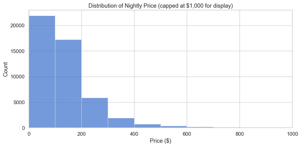
- Log-transformed the heavily skewed price so the model wasn't driven by outliers
- Built ColumnTransformer + Pipeline workflows (scaling, one-hot encoding) to avoid data leakage
- Cleaned Amazon price, discount and rating text into numbers and used a stratified train/test split
What I found
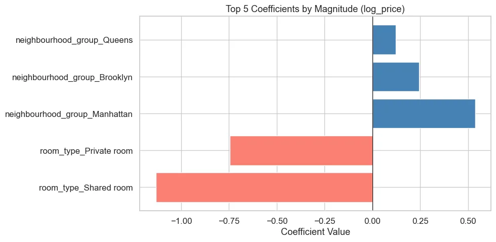
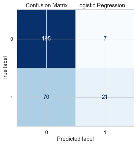
Room type and borough drive price most: Manhattan listings price about 71% above the Bronx. For Amazon, the classifier beat the 31% base rate, but its ROC AUC of 0.65 shows ratings depend on more than price and category. Review text would be the next feature to add.
The Code
The actual Python I wrote for this project. Scroll inside the window to read it all.
# Task A — Airbnb NYC 2019 (Regression)
# # # **Business scenario:** You are helping Airbnb build a suggested-nightly-price tool for new NYC hosts. Predict price from neighborhood, room type, and listing activ

# Imports

import numpy as np                          # numerical computing (log, sqrt, etc.)
import pandas as pd                         # data loading and manipulation
import matplotlib.pyplot as plt             # base plotting library
import seaborn as sns                       # higher-level statistical plots

from sklearn.model_selection import train_test_split        # splits data into train and test sets
from sklearn.linear_model import LinearRegression           # the regression model
from sklearn.preprocessing import OneHotEncoder, StandardScaler  # encode categoricals, scale numerics
from sklearn.compose import ColumnTransformer               # applies different transforms to different columns
from sklearn.pipeline import Pipeline                       # chains preprocessing + model into one object
from sklearn.metrics import r2_score, mean_squared_error    # model evaluation metrics

RANDOM_STATE = 42                           # fixed seed so results are reproducible
pd.set_option('display.max_columns', 50)    # show up to 50 columns in dataframe previews

sns.set_theme(style="whitegrid", palette="muted", font_scale=1.1)  # consistent plot style across all charts
FIGSIZE = (10, 5)                           # standard figure size reused in every plot

airbnb = pd.read_csv('airbnb_nyc_2019.csv')  # load the dataset into a DataFrame
print(airbnb.shape)                           # print (rows, columns) to confirm it loaded correctly
airbnb.head()                                 # display the first 5 rows to inspect the data

# A.1 — Descriptive Analysis
# Report shape, dtypes, missing-value summary, price distribution plot, medians by `neighbourhood_group` and `room_type`, top 5 neighbourhoods by listing count.

# --- Shape and column types ---
print("Shape:", airbnb.shape)       # total number of rows and columns
print("\nColumn types:")             # newline then header label
print(airbnb.dtypes)                 # shows whether each column is numeric, object (text), etc.

# --- Missing value summary ---
missing = airbnb.isnull().sum()                        # count NaN values in each column
missing = missing[missing > 0].sort_values(ascending=False)  # keep only columns that have missing values, sorted
print("\nMissing values:")
print(missing)                       # print the columns with missing counts

# --- Price distribution plot ---
fig, ax = plt.subplots(figsize=FIGSIZE)          # create a figure with our standard size
sns.histplot(airbnb['price'], bins=100, ax=ax)   # histogram of price with 100 bins
ax.set_xlim(0, 1000)                             # cap x-axis at $1,000 so extreme outliers don't compress the chart
ax.set_title('Distribution of Nightly Price (capped at $1,000 for display)')
ax.set_xlabel('Price ($)')
ax.set_ylabel('Count')
plt.tight_layout()                               # prevent labels from being cut off
plt.show()

print(f"\nPrice skewness: {airbnb['price'].skew():.2f}")  # positive skew = long right tail (many cheap, few expensive)

# --- Median prices ---
print(f"\nOverall median price: ${airbnb['price'].median():.2f}")  # median is robust to outliers unlike mean

print("\nMedian price by neighbourhood_group:")
print(airbnb.groupby('neighbourhood_group')['price'].median().sort_values(ascending=False))  # group by borough, get median

print("\nMedian price by room_type:")
print(airbnb.groupby('room_type')['price'].median().sort_values(ascending=False))  # entire home vs private vs shared

# --- Top 5 neighbourhoods by listing count ---
print("\nTop 5 neighbourhoods by listing count:")
print(airbnb['neighbourhood'].value_counts().head())  # value_counts() ranks by frequency, .head() takes top 5

# A.2 — Data Preprocessing
# Drop `price == 0` and cap extreme prices, fill `reviews_per_month` with 0, create `log_price`, split train/test with `random_state=42`.

PRICE_CAP = 500  # listings above $500/night are extreme outliers (<2% of data) that would skew the model

df = airbnb[airbnb['price'] > 0].copy()        # remove $0 listings — likely data errors or free stays
df = df[df['price'] <= PRICE_CAP].copy()        # remove listings above the cap
print(f"Rows after filtering: {len(df)}  (removed {len(airbnb) - len(df)} rows)")

df['reviews_per_month'] = df['reviews_per_month'].fillna(0)  # NaN means no reviews yet, so 0 is the correct value

df['log_price'] = np.log(df['price'])  # log transform makes price more normally distributed, improving linear regression

# Define which columns are categorical vs numeric
CAT_FEATURES = ['neighbourhood_group', 'room_type']          # text columns — will be one-hot encoded
NUM_FEATURES = ['minimum_nights', 'number_of_reviews',       # numeric columns — will be scaled
                'reviews_per_month', 'calculated_host_listings_count', 'availability_365']

X = df[CAT_FEATURES + NUM_FEATURES]   # feature matrix — all input columns
y = df['log_price']                   # target variable — what we want to predict

X_train, X_test, y_train, y_test = train_test_split(
    X, y, test_size=0.2, random_state=RANDOM_STATE  # 80% train, 20% test; fixed seed for reproducibility
)

print(f"Train size: {len(X_train)}, Test size: {len(X_test)}")

# A.3 — Model Building
# Fit a linear regression on `log_price` in a `Pipeline` with a `ColumnTransformer`. Report test R², RMSE on the log scale, and RMSE back-transformed to dollars. Print top 5 coefficients by magnitude.

# ColumnTransformer applies different preprocessing to numeric vs categorical columns
preprocessor = ColumnTransformer(transformers=[
    ('num', StandardScaler(), NUM_FEATURES),                              # scale numerics to mean=0, std=1
    ('cat', OneHotEncoder(handle_unknown='ignore', drop='first'), CAT_FEATURES),  # encode categoricals as 0/1 columns
])                                                                        # drop='first' avoids multicollinearity

# Pipeline chains preprocessing and model so they are fit together (prevents data leakage)
pipeline = Pipeline(steps=[
    ('preprocessor', preprocessor),   # step 1: transform the features
    ('model', LinearRegression()),     # step 2: fit the linear regression
])

pipeline.fit(X_train, y_train)  # fit the entire pipeline on training data only

# --- Evaluate on test set ---
y_pred_log = pipeline.predict(X_test)   # generate predictions on the held-out test set

r2 = r2_score(y_test, y_pred_log)                                          # R²: proportion of variance explained (0–1)
rmse_log = np.sqrt(mean_squared_error(y_test, y_pred_log))                 # RMSE on log scale
rmse_dollars = np.sqrt(mean_squared_error(np.exp(y_test), np.exp(y_pred_log)))  # undo log transform to get dollar error

print(f"Test R\u00b2:             {r2:.4f}")           # higher is better; 1.0 = perfect
print(f"Test RMSE (log $):   {rmse_log:.4f}")      # error in log-dollar units
print(f"Test RMSE (dollars): ${rmse_dollars:.2f}") # average prediction error in actual dollars

# --- Extract and display top 5 coefficients ---
ohe = pipeline.named_steps['preprocessor'].named_transformers_['cat']  # retrieve the fitted OneHotEncoder
cat_feature_names = ohe.get_feature_names_out(CAT_FEATURES).tolist()    # get the generated column names (e.g. room_type_Private)
all_feature_names = NUM_FEATURES + cat_feature_names                    # combine numeric and encoded categorical names

coefs = pipeline.named_steps['model'].coef_                             # array of learned coefficients
coef_df = pd.DataFrame({'feature': all_feature_names, 'coefficient': coefs})  # pair each feature with its coefficient
coef_df['abs_coef'] = coef_df['coefficient'].abs()                      # absolute value for ranking by magnitude
top5 = coef_df.nlargest(5, 'abs_coef')[['feature', 'coefficient']]      # keep top 5 most influential features

print("\nTop 5 coefficients by magnitude:")
print(top5.to_string(index=False))  # print without row numbers for cleaner output

# --- Bar chart of top 5 coefficients ---
fig, ax = plt.subplots(figsize=FIGSIZE)
colors = ['steelblue' if c > 0 else 'salmon' for c in top5['coefficient']]  # blue = raises price, red = lowers price
ax.barh(top5['feature'], top5['coefficient'], color=colors)   # horizontal bar chart
ax.axvline(0, color='black', linewidth=0.8)                   # vertical line at zero for reference
ax.set_title('Top 5 Coefficients by Magnitude (log_price)')
ax.set_xlabel('Coefficient Value')
plt.tight_layout()
plt.show()
# Task B — Amazon Sales (Classification)
# # # **Business scenario:** You are supporting an Amazon category manager who wants to flag products likely to be highly rated (rating ≥ 4.3) for a weekly promotion.
#
# Imports
import numpy as np
import pandas as pd
import matplotlib.pyplot as plt
import seaborn as sns
from sklearn.model_selection import train_test_split # split data into train/test
from sklearn.linear_model import LogisticRegression # our classifier
from sklearn.preprocessing import OneHotEncoder, StandardScaler # feature transformers
from sklearn.compose import ColumnTransformer # apply different transforms per column type
from sklearn.pipeline import Pipeline # chain preprocessing + model into one object
from sklearn.metrics import accuracy_score, roc_auc_score, confusion_matrix, ConfusionMatrixDisplay
RANDOM_STATE = 42 # ensures reproducibility everywhere
pd.set_option('display.max_columns', 50)
# Apply a consistent visual theme to all plots (per project style guide)
sns.set_theme(style="whitegrid", palette="muted", font_scale=1.1)
PLT_FIGSIZE = (9, 5) # shared figure size used across all charts
# Load the dataset from the same folder as this notebook
amazon = pd.read_csv('amazon_sales.csv')
print(amazon.shape) # (rows, columns)
amazon.head() # preview first 5 rows
# B.1 — Descriptive Analysis
# Clean `discounted_price`, `actual_price`, `discount_percentage`, `rating`, `rating_count` into numeric types. Create a `top_category` column. Report mean/median rating, category counts, and the base rate of `rating >= 4.3`.
# ── B.1 Descriptive Analysis ─────────────────────────────────────────────────
# Convert price columns to float (they are already numeric in this dataset)
amazon['discounted_price'] = pd.to_numeric(amazon['discounted_price'], errors='coerce')
amazon['actual_price'] = pd.to_numeric(amazon['actual_price'], errors='coerce')
# Remove the '%' sign from discount_percentage, then convert to float
amazon['discount_percentage'] = (
amazon['discount_percentage']
.astype(str)
.str.replace('%', '', regex=False)
)
amazon['discount_percentage'] = pd.to_numeric(amazon['discount_percentage'], errors='coerce')
# Convert rating and rating_count to numeric (coerce turns non-numeric into NaN)
amazon['rating'] = pd.to_numeric(amazon['rating'], errors='coerce')
amazon['rating_count'] = pd.to_numeric(amazon['rating_count'], errors='coerce')
# Extract the top-level category (the text before the first '|')
# e.g. "Computers&Accessories|Cables|..." → "Computers&Accessories"
amazon['top_category'] = amazon['category'].str.split('|').str[0]
# ── Summary statistics ────────────────────────────────────────────────────────
print("=== Rating stats ===")
print(f" Mean rating : {amazon['rating'].mean():.3f}")
print(f" Median rating : {amazon['rating'].median():.1f}")
print()
print("=== Products per top category ===")
print(amazon['top_category'].value_counts())
print()
# Base rate = share of products that are "highly rated" (our positive class)
base_rate = (amazon['rating'] >= 4.3).mean()
print(f"=== Base rate (rating >= 4.3) : {base_rate:.4f} ({base_rate*100:.1f}%) ===")
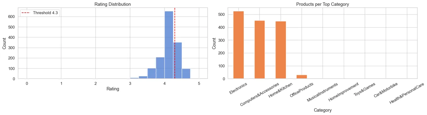
# ── Visualizations ────────────────────────────────────────────────────────────
fig, axes = plt.subplots(1, 2, figsize=(PLT_FIGSIZE[0] * 2, PLT_FIGSIZE[1]))
# Left plot: distribution of ratings with the 4.3 threshold marked
axes[0].set_title("Rating Distribution")
sns.histplot(amazon['rating'].dropna(), bins=20, ax=axes[0],
color=sns.color_palette("muted")[0])
axes[0].axvline(4.3, color='red', linestyle='--', label='Threshold 4.3')
axes[0].set_xlabel("Rating")
axes[0].set_ylabel("Count")
axes[0].legend()
# Right plot: how many products fall in each top-level category
axes[1].set_title("Products per Top Category")
amazon['top_category'].value_counts().plot(
kind='bar', ax=axes[1], color=sns.color_palette("muted")[1])
axes[1].set_xlabel("Category")
axes[1].set_ylabel("Count")
axes[1].tick_params(axis='x', rotation=30)
plt.tight_layout()
plt.show()
# B.2 — Data Preprocessing
# Create `high_rated`, log-transform `rating_count`, drop NaNs in the feature set, split train/test with `random_state=42` and `stratify=y`.
# ── B.2 Data Preprocessing ───────────────────────────────────────────────────
# Create binary target: 1 = high-rated (rating >= 4.3), 0 = not high-rated
amazon['high_rated'] = (amazon['rating'] >= 4.3).astype(int)
# Log-transform rating_count to reduce right skew
# np.log1p = log(1 + x), which safely handles zeros
amazon['log_rating_count'] = np.log1p(amazon['rating_count'])
# Select the features we'll feed into the model
features = ['discounted_price', 'actual_price', 'discount_percentage',
'log_rating_count', 'top_category']
target = 'high_rated'
# Drop any rows that have missing values in our feature set
model_df = amazon[features + [target]].dropna()
print(f"Rows after dropping NaNs: {len(model_df)}")
X = model_df[features]
y = model_df[target]
# Split 80% train / 20% test
# stratify=y keeps the same class ratio in both splits (important for imbalanced data)
X_train, X_test, y_train, y_test = train_test_split(
X, y, test_size=0.2, random_state=RANDOM_STATE, stratify=y
)
print(f"Train size: {len(X_train)} | Test size: {len(X_test)}")
print(f"Train positive rate: {y_train.mean():.4f} | Test positive rate: {y_test.mean():.4f}")
# B.3 — Model Building
# Build a `Pipeline` with `ColumnTransformer` (scale numeric, one-hot `top_category`) + `LogisticRegression(max_iter=2000)`. Report test accuracy, ROC AUC, confusion matrix. Print top 5 coefficients by magnitude.
# ── B.3 Model Building ───────────────────────────────────────────────────────
# Define which columns are numeric and which are categorical
numeric_features = ['discounted_price', 'actual_price', 'discount_percentage', 'log_rating_count']
categorical_features = ['top_category']
# ColumnTransformer applies a different transformation to each column group:
# - StandardScaler: rescales numeric columns to mean=0, std=1
# - OneHotEncoder: converts top_category into binary dummy columns
preprocessor = ColumnTransformer(transformers=[
('num', StandardScaler(), numeric_features),
('cat', OneHotEncoder(handle_unknown='ignore'), categorical_features),
])
# Pipeline chains preprocessing + classifier so they are fit and predict together,
# preventing data leakage (scaler/encoder only learn from training data)
pipeline = Pipeline(steps=[
('preprocessor', preprocessor),
('classifier', LogisticRegression(max_iter=2000, random_state=RANDOM_STATE)),
])
# Train the model
pipeline.fit(X_train, y_train)
# Generate predictions and probability scores on the held-out test set
y_pred = pipeline.predict(X_test)
y_proba = pipeline.predict_proba(X_test)[:, 1] # probability of class 1
# ── Performance metrics ───────────────────────────────────────────────────────
acc = accuracy_score(y_test, y_pred)
auc = roc_auc_score(y_test, y_proba)
print(f"Test Accuracy : {acc:.4f}")
print(f"Test ROC AUC : {auc:.4f}")
# ── Confusion matrix ──────────────────────────────────────────────────────────
# Shows counts of: True Negatives | False Positives
# False Negatives | True Positives
fig, ax = plt.subplots(figsize=PLT_FIGSIZE)
ConfusionMatrixDisplay.from_predictions(y_test, y_pred, ax=ax,
colorbar=False, cmap='Blues')
ax.set_title("Confusion Matrix — Logistic Regression")
plt.tight_layout()
plt.show()
# ── Top 5 coefficients by magnitude ──────────────────────────────────────────
# Extract the fitted logistic regression from the pipeline
lr_model = pipeline.named_steps['classifier']
# Get the feature names that OneHotEncoder created for top_category
ohe_cols = (pipeline.named_steps['preprocessor']
.named_transformers_['cat']
.get_feature_names_out(categorical_features)
.tolist())
all_features = numeric_features + ohe_cols
# Pair each feature name with its coefficient; larger |coef| = stronger influence
coef_df = pd.DataFrame({'feature': all_features, 'coefficient': lr_model.coef_[0]})
coef_df['abs_coef'] = coef_df['coefficient'].abs()
top5 = coef_df.nlargest(5, 'abs_coef')
print("\nTop 5 coefficients by magnitude:")
print(top5[['feature', 'coefficient']].to_string(index=False))
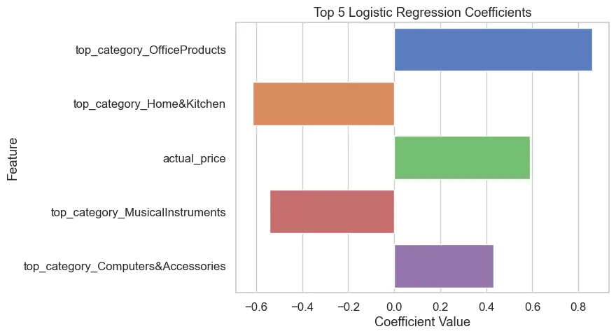
# Bar chart of top 5 coefficients
fig, ax = plt.subplots(figsize=PLT_FIGSIZE)
sns.barplot(data=top5, x='coefficient', y='feature', palette='muted', ax=ax)
ax.set_title("Top 5 Logistic Regression Coefficients")
ax.set_xlabel("Coefficient Value")
ax.set_ylabel("Feature")
plt.tight_layout()
plt.show()