Overview
An executive team was weighing an investment in Bitcoin and wanted to know how the market felt about it. I ran a sentiment analysis on Bitcoin tweets to measure emotion and tone, and turned it into a recommendation.
Key results
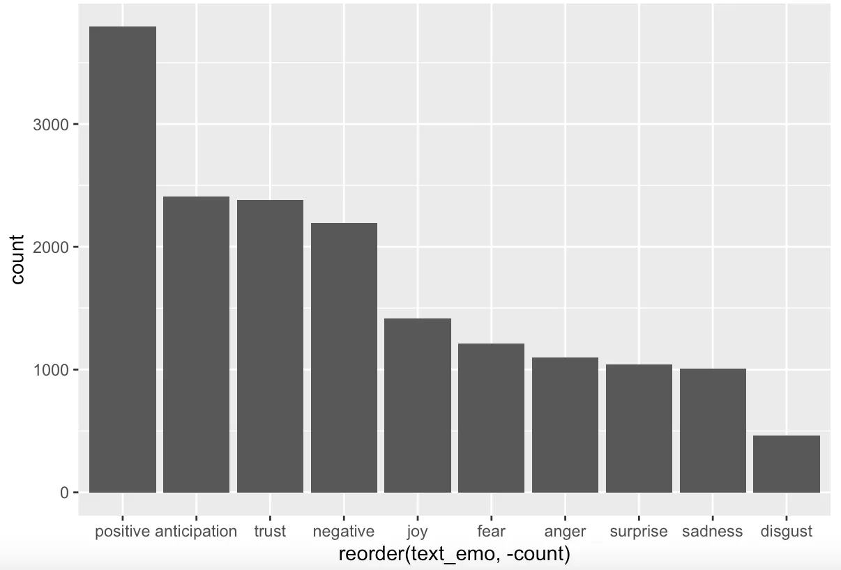
3,794positive-sentiment words vs. 2,193 negative
2,410anticipation signals, the strongest emotion in the data
2,383trust signals, close behind anticipation
2lexicons compared: NRC emotions and Bing positive/negative
The question
Is public conversation about Bitcoin optimistic or fearful, and what words drive each side?
What I did
- Built a term-document matrix and charted the most frequent words, plus a word cloud
- Scored every tweet against the NRC lexicon (syuzhet) across eight emotions
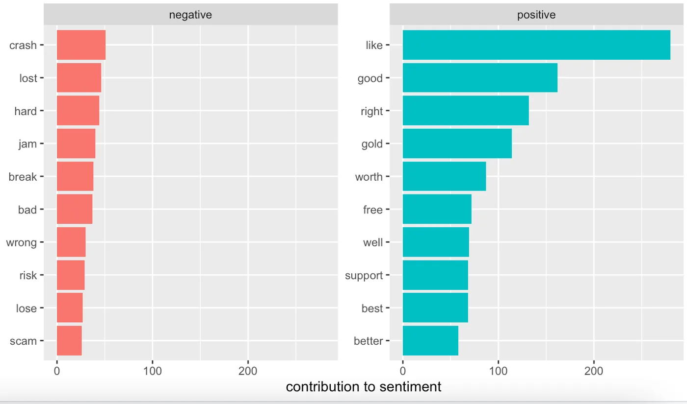
- Tokenized the text with tidytext and joined it to the Bing lexicon to rank the top positive and negative words
- Translated the results into an investment recommendation for executives
What I found
Positive language outweighed negative by a wide margin, led by anticipation and trust. The top negative words (crash, lost, risk, scam) point to the fears to watch. I recommended entering while interest was high and treating dips as buying opportunities, while monitoring negative sentiment as an early warning.
The Code
The actual R I wrote for this project. Scroll inside the window to read it all.
install.packages("tm")
install.packages("SnowballC")
install.packages("wordcloud")
install.packages("RColorBrewer")
install.packages("syuzhet")
install.packages("tidytext")
install.packages("tidyverse")

library("tm")
library("SnowballC")
library("wordcloud")
library("RColorBrewer")
library("syuzhet")
library("tidytext")
library("tidyverse")


tweets <- read.csv("Desktop/tweets.csv", header= TRUE, sep = ",", quote = '"')
tweets
head(tweets)
summary(tweets)

##### term document matrix ####

dtm <- TermDocumentMatrix(tweets)
dtm_m <- as.matrix(dtm)

#sort by decreasing value of frequency
dtm_s <- sort(rowSums(dtm_m), decreasing = TRUE)
dtm_d <-data.frame(word = names(dtm_s), freq = dtm_s)

#display top 10 most frequent words
head(dtm_d, 10)

#plotting top 10 words
barplot(dtm_d[1:10,]$freq, las = 2, names.arg = dtm_d[1:10,]$word,
        col = "lightgreen", main = "top 10 most frequent words",
        ylab = "word frequencies")


########## word cloud ##########

set.seed(1234)

wordcloud(words = dtm_d$word, freq = dtm_d$freq, min.freq = 5,
          max.words = 100, random.order = FALSE, rot.per = 0.4,
          colors = brewer.pal(8, "Dark2"))

########### Sentiment Analysis: part 1 ##########
#Syuzhet package
colnames(tweets)

text_reviews <- tibble(text = str_to_lower(tweets$text))

text_emo <- get_nrc_sentiment(text_reviews$text)
text_emo

text_emo_sum <- colSums(text_emo)
text_emo_sum

text_emo_df <- data.frame(count = text_emo_sum,
                          text_emo = names(text_emo_sum))
text_emo_df

#### create bar plot ####

ggplot(text_emo_df, aes(x= reorder(text_emo,-count),
                        y= count)) + geom_bar(stat = 'identity')


########## sentiment analysis: part 2 ##########
#bing lexicon

bing_counts <- text_reviews %>% unnest_tokens(output = word,input = text)
bing_counts

bing_counts <- text_reviews %>%
  unnest_tokens(output = word,input = text) %>%
  inner_join(get_sentiments("bing")) %>%
               count(word,sentiment,sort=TRUE)

bingtop <- bing_counts %>% group_by(sentiment) %>%
  slice_max(order_by = n, n=10) %>%
  ungroup() %>%
  mutate(word= reorder(word,n))
bingtop

bingtop %>% ggplot(aes(word,n, fill= sentiment))+
  geom_col(show.legend = FALSE)+
  facet_wrap(~sentiment, scales = "free_y")+ labs(y= "contribution to sentiment",x= NULL)+
  coord_flip()