Overview
A gas station owner wanted to understand how competitor pricing and seasonality affect her sales. I forecast next week's demand and used regression to recommend a price for each competitor scenario.
Key results
962 galforecast average daily sales for the next week (range 847–1,077)
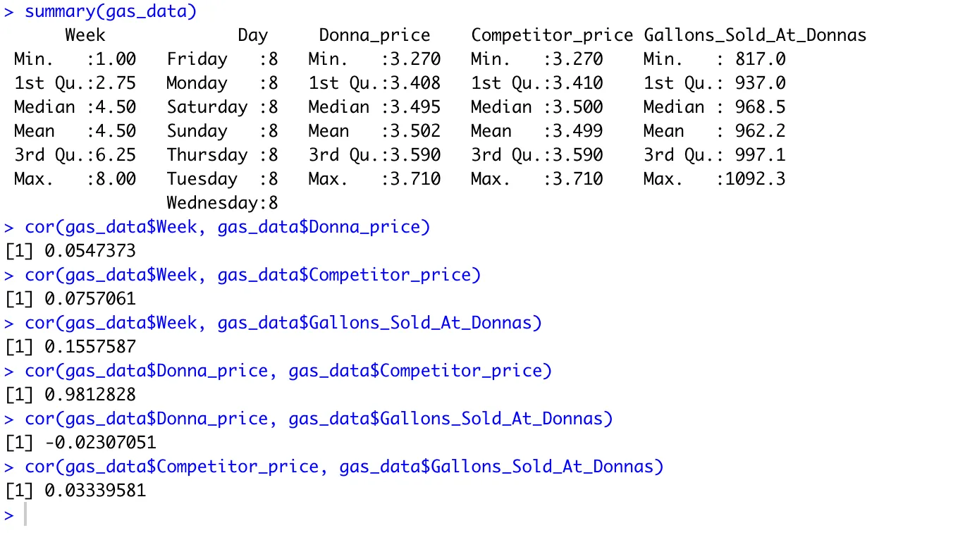
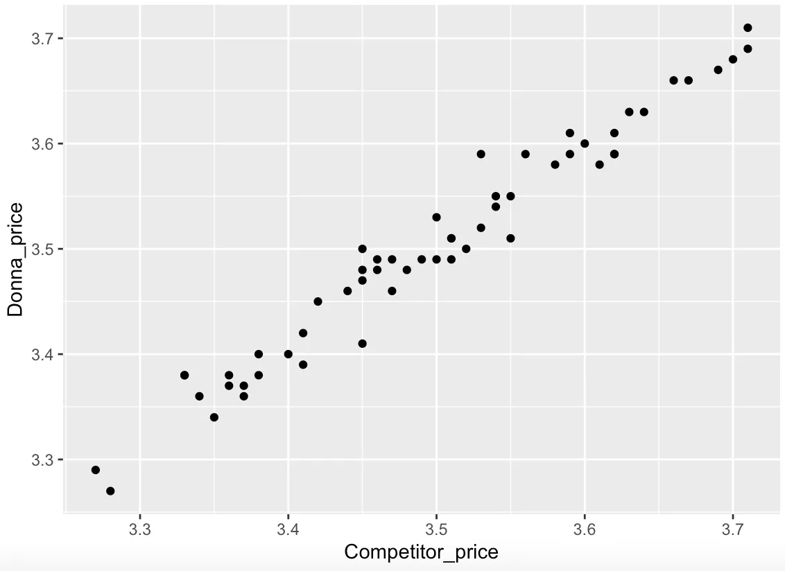
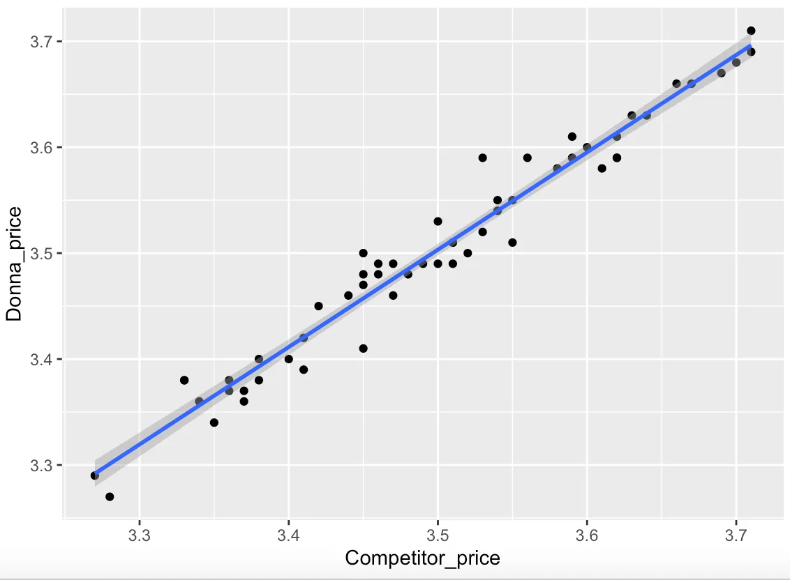
R² 0.96for Donna's price vs. her competitor's price (correlation 0.981)
$3.49recommended price when the competitor sits at its $3.50 average
56 daysof daily sales and price data analyzed
The question
How should Donna price her gas to sell the most gallons when her competitor's price is at its low, average or high?
What I did
- Explored eight weeks of daily price and volume data for trends and correlations
- Forecast sales for days 57–63 with a range of likely outcomes
- Ran simple and multiple regressions on Donna's price, the competitor's price and gallons sold
- Checked results for bias and potential problems before recommending
What I found
Donna's prices track her competitor's almost exactly. The best strategy is to price just under the competitor at average and high prices ($3.49 vs. $3.50, $3.68 vs. $3.71), but slightly above when the competitor drops to its low ($3.28 vs. $3.27).
The Code
The actual R I wrote for this project. Scroll inside the window to read it all.
#install packages
#tidverse-- allows you to use the pipe operator
#ggplot----- alows for graphs
#janitor----- cleans variable names
install.packages("tidyverse")
install.packages("ggplot2")
install.packages("janitor")
#load packages
library(tidyverse)
library(ggplot2)
library(janitor)
library(car)
library(gridExtra)
library(forecast)
library(fpp2)

##### load data#####
# getwd ---- identifies our working directory
#read.csv("df.csv", header = TRUE, sep=",", quote= '"')
gas_data <- read.csv("Desktop/DonnasGasStation.csv", header= TRUE, sep = ",", quote = '"')

gas_data
#######Data clean up######
clean_names(gas_data)
colnames(gas_data)

##renaming variables
names(gas_data)[3] <- "Donna_price"
names(gas_data)[4] <- "Competitor_price"
names(gas_data)[5] <- "Gallons_Sold_At_Donnas"
#summary
summary(gas_data)

#dimension of data
dim(gas_data)

# structure of the data
str(gas_data)

#first 6 rows of data
head(gas_data)

#display a certain column
gas_data$Week

#display a table of a column
table(gas_data$Day)

table(gas_data$Week, gas_data$Day)
table(gas_data$Donna_price, gas_data$Day)
table(gas_data$Competitor_price, gas_data$Day)

table(gas_data$Donna_price, gas_data$Week)
table(gas_data$Competitor_price, gas_data$Week)


#nicer way to display a table
Week_count <- count(gas_data,'Week')
Week_count


#scatterplots
#Donnas prices on each day
ggplot(data = gas_data) +
geom_point(mapping = aes(x = Day, y = Donna_price))
#Gallons sold at each of donnas prices
ggplot(data = gas_data) +
  geom_point(mapping = aes(x = Donna_price, y = Gallons_Sold_At_Donnas))


##########

##########num 1 clean data
clean_names(gas_data)
colnames(gas_data)
names(gas_data)[3] <- "Donna_price"
names(gas_data)[4] <- "Competitor_price"
names(gas_data)[5] <- "Gallons_Sold_At_Donnas"
##########num 2 five num summary
summary(gas_data)
##########num 3 table for each column
table(gas_data$Week)
table(gas_data$Day)
table(gas_data$Donna_price)
table(gas_data$Competitor_price)
table(gas_data$Gallons_Sold_At_Donnas)
##########num 4 histogram/box plots for 2 columns
ggplot(data = gas_data) + geom_histogram(aes(x= Competitor_price))
ggplot(data = gas_data) + geom_histogram(aes(x= Donna_price))
##########num 5 histogram with color and shape
ggplot(data = gas_data) + geom_histogram(aes(x=Donna_price), color = "red", fill = "pink")
##########num 6 bar graph
ggplot(data = gas_data) + geom_bar(mapping = aes(x = Donna_price))
ggplot(data = gas_data) + geom_bar(mapping = aes(x = Competitor_price))

##########num 7 dodge bar
ggplot(data = gas_data) +
  geom_bar(mapping = aes(x = Donna_price,fill=Day), position="dodge")

ggplot(data = gas_data) +
  geom_bar(mapping = aes(x = Competitor_price,fill=Day), position="dodge")

##########num 8 scatter plot with trend line
ggplot(data = gas_data, mapping = aes(x = Donna_price, y = Gallons_Sold_At_Donnas)) +
  geom_point(mapping = aes(color = Day))+
  geom_smooth()

ggplot(data = gas_data, mapping = aes(x = Competitor_price, y = Gallons_Sold_At_Donnas)) +
  geom_point(mapping = aes(color = Day))+
  geom_smooth()

ggplot(data = gas_data, mapping = aes(x = Competitor_price, y = Donna_price)) +
  geom_point(mapping = aes(color = Day))+
  geom_smooth()

##########num 9 facet graph
ggplot(data= gas_data)+
  geom_point(mapping=aes(x=Donna_price,y=Gallons_Sold_At_Donnas,color=Day))+
  facet_wrap(~Week)
##############################################
##############################################
plot(gas_data$Gallons_Sold_At_Donnas)

ggplot(data= gas_data, aes(x= Gallons_Sold_At_Donnas, y = Donna_price)) + geom_line()

summary(gas_data)

# correlation number
# format:cor(df$var1, df$var2)

cor(gas_data$Week, gas_data$Donna_price)
cor(gas_data$Week, gas_data$Competitor_price)
cor(gas_data$Week, gas_data$Gallons_Sold_At_Donnas)

cor(gas_data$Donna_price, gas_data$Competitor_price)
cor(gas_data$Donna_price, gas_data$Gallons_Sold_At_Donnas)

cor(gas_data$Competitor_price, gas_data$Gallons_Sold_At_Donnas)


##### plot #####
plot_DPrice <- ggplot(gas_data, aes(x= Competitor_price, y= Donna_price)) + geom_point()
plot_DPrice

plot_DPrice_r <- plot_DPrice + geom_smooth(method= 'lm')
plot_DPrice_r

##### Simple Regression #####

#competitor price and donnas price becuase best correlation

#build model
model_1 <- lm(Donna_price ~ Competitor_price, gas_data)
# print summary of model
summary(model_1)

# prediction
#pred_frame_1 <- data.frame(Competitor_price = c(3.56, 3.66))
#predict(model_1, newdata = pred_frame_1)

pred_frame_1 <- data.frame(Competitor_price = c(3.270, 3.410, 3.500, 3.590, 3.710))
predict(model_1, newdata = pred_frame_1)

##### Multiple Regression #####
summary(gas_data)
model_2 <- lm(Donna_price ~ Competitor_price + Gallons_Sold_At_Donnas, data = gas_data)
summary(model_2)

#prediction
#pred_frame_2 <- data.frame(Competitor_price= c(3.55, 3.66), Gallons_Sold_At_Donnas=c(968.5, 968.5))
#predict(model_2, newdata = pred_frame_2)

#comp price max and gas sold at min avg max
pred_frame_2 <- data.frame(Competitor_price= c(3.71, 3.71, 3.71), Gallons_Sold_At_Donnas=c(817.0, 962.2, 1092.3))
predict(model_2, newdata = pred_frame_2)

#comp price avg and gas sold at min avg max
pred_frame_3 <- data.frame(Competitor_price= c(3.499, 3.499, 3.499), Gallons_Sold_At_Donnas=c(817.0, 962.2, 1092.3))
predict(model_2, newdata = pred_frame_3)

#comp price min and gas sold at min avg max
pred_frame_4 <- data.frame(Competitor_price= c(3.270, 3.270, 3.270), Gallons_Sold_At_Donnas=c(817.0, 962.2, 1092.3))
predict(model_2, newdata = pred_frame_4)
####################
####################

#####time series#####
#data in time series
Gas_ts <- ts(gas_data$Gallons_Sold_At_Donnas, start = c(1,1), frequency = 1)

#verify its a time series
str(Gas_ts)

#plot time series
plot(Gas_ts)

######moving average forecast
#build moving avg model looking at all 56 days in the past
Gas_MA <- ma(Gas_ts, order= 1, centre=FALSE)
Gas_MA

Gas_MA_fcst <- forecast(Gas_MA, h=7)
Gas_MA_fcst
plot(Gas_MA_fcst)
install.packages("tidyverse")
install.packages("car")
install.packages("ggplot2")
install.packages("gridExtra")
library("tidyverse")
library("car") #gives us regression packages
library("ggplot2")
library("gridExtra")
insurance <- read.csv("Desktop/Insurance.csv", header= TRUE, sep = ",", quote = '"')
insurance
########## prelim exploration ##########
head(insurance)
tail(insurance)
str(insurance)
summary(insurance)
##### plots
# format: ggplot(df, aes(x=var 1, y=var 2)) + geom_point()
# Plot age vs charges
plot_age <- ggplot(insurance, aes(x= age, y= charges)) + geom_point()
plot_age
# correlation number
# format:cor(df$var1, df$var2)
cor(insurance$age, insurance$charges)
# plot region vs charges
plot_region <- ggplot(insurance, aes(x= region, y= charges)) + geom_point()
plot_region
#plot bmi vs charges
plot_bmi <- ggplot(insurance, aes(x= bmi, y= charges)) + geom_point()
plot_bmi
########## simple regression ##########
# plot regression line
# format: regular plot + geom_smooth(method = 'lm')
## identify if age is a good predictor of charges
plot_age_r <- plot_age + geom_smooth(method= 'lm')
plot_age_r
#build regression model
# format: lm(dependent var, ~ predictor var 1, data = df)
mod1 <- lm(charges ~ age, data = insurance)
# show output
summary(mod1)
#make prediction
#First create a dataframe
# predict age of 22, 32, 52
pred_1 <- data.frame(age= c(22,32, 52))
# prediciton output
predict(mod1, newdata = pred_1)
########## multiple regression ##########
str(insurance)
# convert categorical variables into factors
# format: df$variable <- as.factor(df$variable)
#change sex to factor
insurance$sex <- as.factor(insurance$sex)
#change smoker to facor
insurance$smoker <- as.factor(insurance$smoker)
#change region to facor
insurance$region <- as.factor(insurance$region)
##### build MR (multiple regression model) with age + BMI #####
# format: lm(dependent var, ~ predictor var 1 + predictor var 2, data = df)
mod2 <- lm(charges ~ age + bmi, data = insurance)
summary(mod2)
#prediction
# create dataframe
pred_2 <- data.frame(age= c(22, 25, 52), bmi= c(36, 31, 23))
#predict
predict(mod2, newdata = pred_2)
##### build model with all predictors #####
mod3 <- lm(charges ~ age + bmi + smoker + children + sex + region, data = insurance)
summary(mod3)
#####since sex has p vlaue > .05, remove from model#####
mod4 <- lm(charges ~ age + bmi + smoker + children + region, data = insurance)
summary(mod4)
#prediction
#create dataframe
pred_3 <- data.frame(age= c(25, 25), bmi = c(31, 18), smoker= c("yes", "no"), children = c(4, 2), region = c("southwest", "southwest"))
#predict
predict(mod4, newdata = pred_3)
summary(insurance)