Overview
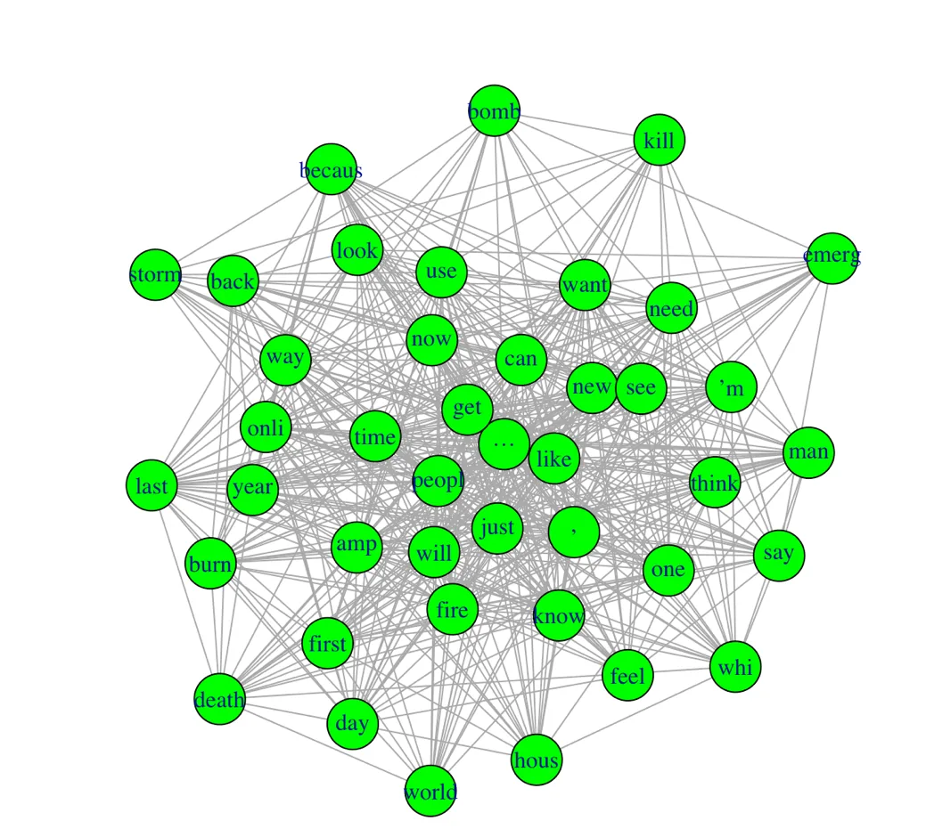
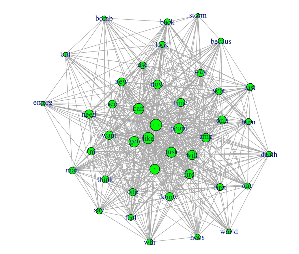
Inspired by a post-apocalyptic TV show, I asked which words a company selling emergency supplies should use to reach "doomsday prepper" customers. I built a word network from tweets about real-world disasters.
Key results
1,500disaster tweets randomly sampled from a larger Kaggle dataset
bomb ↔ killone of the strongest word connections, alongside death ↔ burn
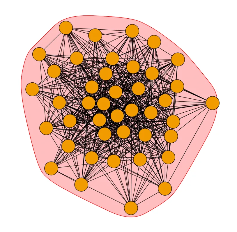
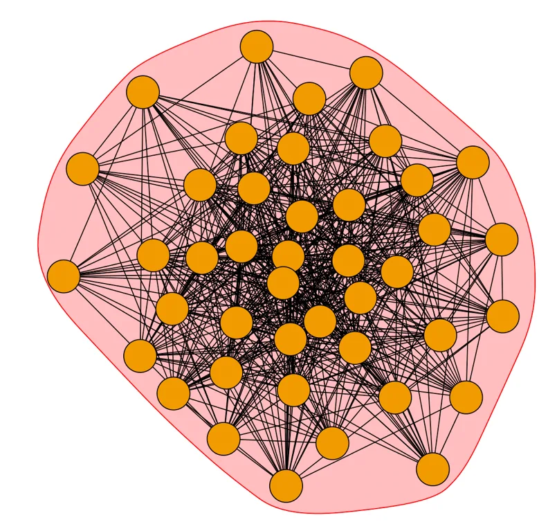
1tightly connected community: nearly every word links within a few steps
The question
Which disaster-related words appear together, and what does that say about effective marketing language for emergency-preparedness products?
What I did
- Cleaned the text: removed URLs, symbols, numbers, punctuation and stop words, then stemmed words
- Built a term-document matrix and kept words appearing more than 25 times
- Converted co-occurrence into an adjacency matrix and graphed it with igraph
- Ran community detection to test how clustered the vocabulary was
What I found
The vocabulary is so interconnected that almost any disaster word reaches the others in a step or two, so marketing language can touch many scenarios at once. Interestingly, "storm" and "emergency" sat at opposite ends of the network. I applied the same network techniques to a car-tire ratings dataset.
The Code
The actual R I wrote for this project. Scroll inside the window to read it all.
install.packages("tm")
install.packages("SnowballC")
install.packages("wordcloud")
install.packages("RColorBrewer")
install.packages("syuzhet")
install.packages("tidytext")
install.packages("tidyverse")
install.packages("igraph")

library("tm")
library("SnowballC")
library("wordcloud")
library("RColorBrewer")
library("syuzhet")
library("tidytext")
library("tidyverse")
library("igraph")

worldevents <- read.csv("Desktop/worldevents2.csv", header= TRUE, sep = ",", quote = '"')
worldevents
head(worldevents)

#clean and data prep
TextDoc <- Corpus(VectorSource(worldevents$text))
#replace special characters with space
toSpace <- content_transformer(function (x,pattern)gsub(pattern,
                                                        "",x))
TextDoc <-tm_map(TextDoc,toSpace,"/")
TextDoc <-tm_map(TextDoc,toSpace,"@")
TextDoc <-tm_map(TextDoc,toSpace,"\\|")

#convert text to lowercase
TextDoc <-tm_map(TextDoc,tolower)
#remove numbers
TextDoc <-tm_map(TextDoc,removeNumbers)
#remove punctuation
TextDoc <-tm_map(TextDoc,removePunctuation)

#stemming... transforming words to their base words
TextDoc <-tm_map(TextDoc,stemDocument)

#remove common stop words
TextDoc <-tm_map(TextDoc,removeWords,stopwords("english"))

#remove URLS
removeURL <- function(x) gsub ('http[[:alnum:]]*','',x)
TextDoc <-tm_map(TextDoc,content_transformer(removeURL))

#remove specific words
TextDoc <-tm_map(TextDoc,removeWords, c('book', 'read'))


TextDoc <-tm_map(TextDoc,stripWhitespace)

#term document matrix
tdm <- TermDocumentMatrix(TextDoc)
tdm <- as.matrix(tdm)

#reduce size of tdm
tdm <- tdm[rowSums(tdm) >25,]

#show first 10 text words

tdm[1:10,1:10]

######## create network
tdm[tdm >1] <-1
#transpose the tdm matrix

termM <- tdm %*% t(tdm)
termM[1:10, 1:10]

g <- graph.adjacency(termM, weighted = T, mode= 'undirected')
g
g <- simplify(g)
g

#label vertex
V(g)$label <- V(g)$name
V(g)$label

#add wight
V(g)$degree <- degree(g)
V(g)$degree

#histogram of verticies weight
hist(V(g)$degree, col = 'green')

#plot network
set.seed(100)
plot(g, vertex.color= 'green')

#network graph weight
plot(g,
     vertex.color = 'green',
     vertex.size = V(g)$degree*(0.25),
     edge.arrow.size = 0.1,
     layout = layout.fruchterman.reingold)


########### community detection

ComDec1 <- cluster_edge_betweenness(g)
plot (ComDec1,g)

ComDec2 <- cluster_label_prop(g)
plot(ComDec2,g)

# highlight degrees
V(g)$label.cex <- 2*V(g)$degree/max(V(g)$degree) + 0.3
V(g)$label.color <- rgb(0,0,.2,.8)
V(g)$frame.color <- NA
egam <- (E(g)$weight+0.4)/max(E(g)+0.4)
E(g)$color <- rgb(.5,.5,0,.8)
E(g)$width <- egam

plot(g, vertex.color = 'green',
     vertex.size = V(g)$degree*.7)
install.packages("igraph")
library("igraph")
#load data
tires <- read.csv("Desktop/tires1.csv", header= TRUE, sep = ",", quote = '"')
tires
head(tires)
x <- data.frame(tires$Model, tires$Rating)
head(x)
#create network connections
net <- graph.data.frame(x, directed = T)
net
#verticies
V(net)
#label vertices
V(net)$label <-V(net)$name
V(net)$label
#add weight/degree
V(net)$degree <- degree(net)
V(net)$degree
plot(net, vertex.color = "green",
vertex.size = 3,
edge.arrow.size= .3)
#comunity detection
ComDec <- cluster_edge_betweenness(net)
plot(ComDec, net)