Overview
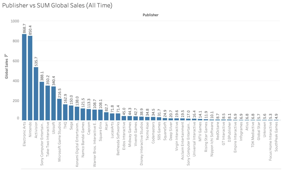
This was the capstone for my Business Analytics certificate. Using decades of video game sales data, I identified the top publishers, the genres and regions where each one dominates, and forecast their next five years of sales.
Key results
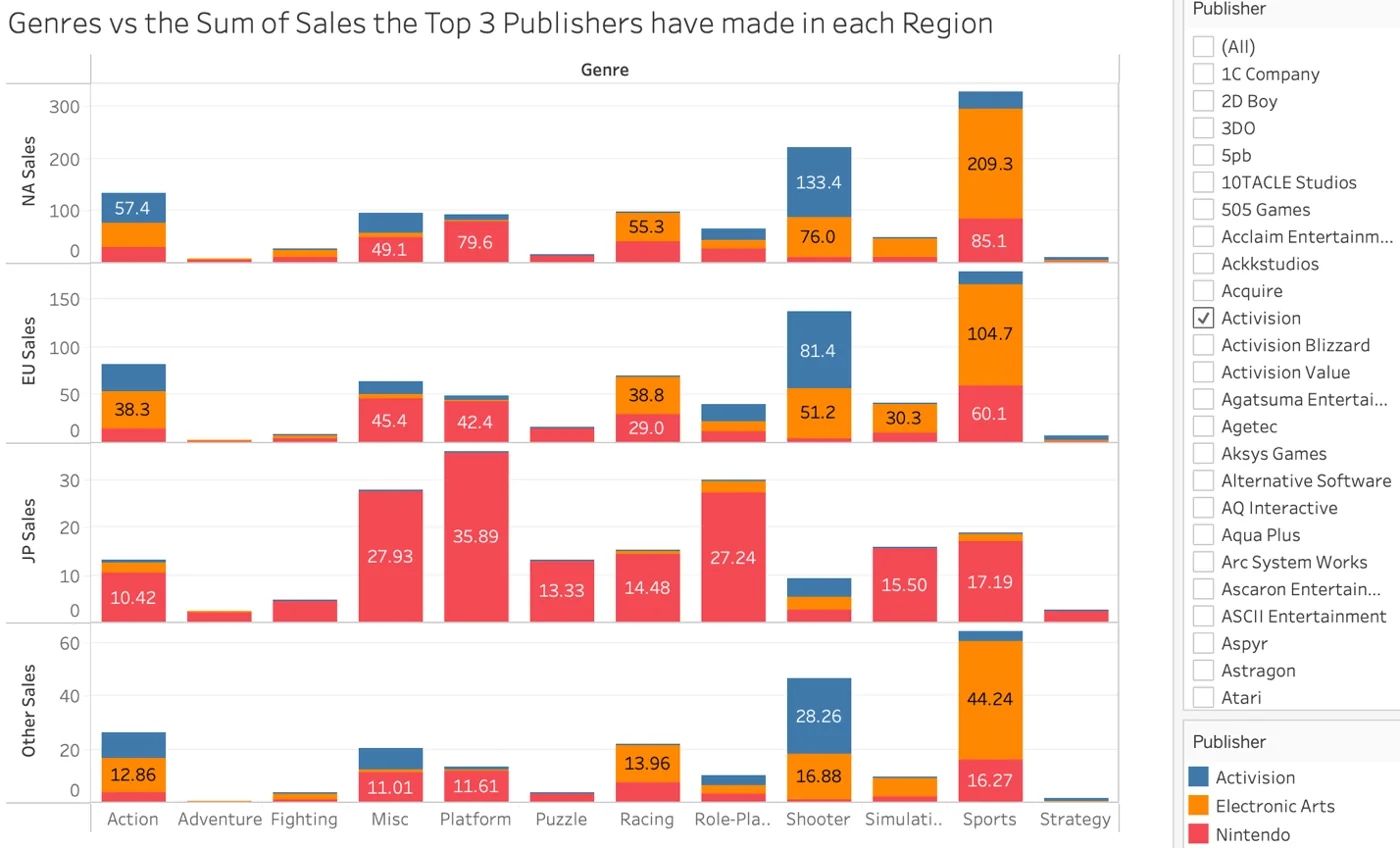
209.3MEA sports sales in North America, the biggest publisher-genre pairing
133.4MActivision shooter sales in North America
>90%Nintendo's sales lead over EA and Activision across every genre in Japan
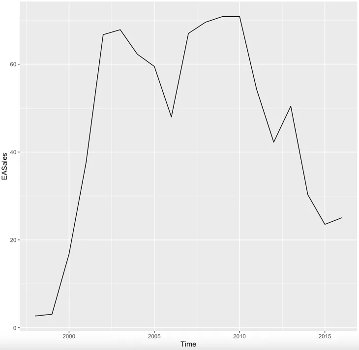
82Mprojected record year for EA, the strongest of the three forecasts
The question
Which publishers lead the market, which genres and regions they're strongest in, and who is best positioned for the next five years?
What I did
- Explored genre trends against critic and user scores, and found that reviews don't predict sales
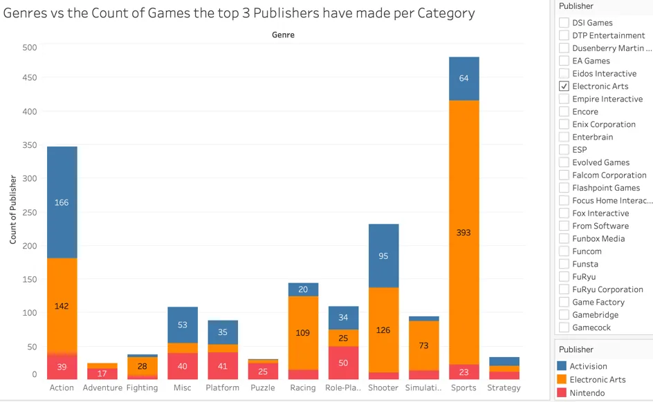
- Ranked publishers by global sales, then broke the top three down by genre and region (NA, EU, JP, Other)
- Built a yearly global-sales time series for each publisher
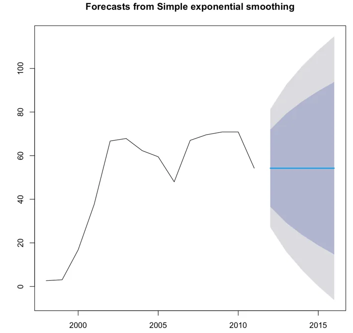
- Forecast five years ahead with exponential smoothing and moving averages in R
What I found
EA, Nintendo and Activision lead overall, but each wins different ground: EA in sports, Activision in shooters, Nintendo in Japan. The forecasts put EA in the strongest position and Nintendo in the weakest, which surprised me given Nintendo's history.
The Code
The actual R I wrote for this project. Scroll inside the window to read it all.
#install packages
#tidverse-- allows you to use the pipe operator
#ggplot----- alows for graphs
#janitor----- cleans variable names
install.packages("tidyverse")
install.packages("ggplot2")
install.packages("janitor")
install.packages("car")
install.packages("gridExtra")
install.packages("forecast")
install.packages("fpp2")
install.packages('TSstudio')
#load packages
library(tidyverse)
library(ggplot2)
library(janitor)
library(car)
library(gridExtra)
library(forecast)
library(fpp2)
library(TSstudio)

vgames <- read.csv("Desktop/VideoGameSales.csv", header= TRUE, sep = ",", quote = '"')

vgames

#summary
summary(vgames)

#dimension of data
dim(vgames)

# structure of the data
str(vgames)

#first 6 rows of data
head(vgames)

#table of each column im using
table(vgames$Genre)
table(vgames$Publisher)
table(vgames$NA_Sales)
table(vgames$EU_Sales)
table(vgames$JP_Sales)
table(vgames$Other_Sales)

#correlation number
cor(vgames$Critic_Score, vgames$NA_Sales)
cor(vgames$Critic_Score, vgames$EU_Sales)
cor(vgames$Critic_Score, vgames$JP_Sales)
cor(vgames$User_Score, vgames$NA_Sales)
cor(vgames$User_Score, vgames$EU_Sales)
cor(vgames$User_Score, vgames$JP_Sales)

cor(vgames$EU_Sales, vgames$NA_Sales)
cor(vgames$EU_Sales, vgames$JP_Sales)
cor(vgames$JP_Sales, vgames$NA_Sales)
cor(vgames$Other_Sales, vgames$NA_Sales)
cor(vgames$Other_Sales, vgames$EU_Sales)
cor(vgames$Other_Sales, vgames$JP_Sales)

cor(vgames$NA_Sales, vgames$EU_Sales)

##### plots
plot_NAsales <- ggplot(vgames, aes(x= EU_Sales, y= NA_Sales)) + geom_point()
plot_NAsales

plot_NAsales_r <- plot_NAsales + geom_smooth(method= 'lm')
plot_NAsales_r
#install packages
#tidverse-- allows you to use the pipe operator
#ggplot----- alows for graphs
#janitor----- cleans variable names
install.packages("tidyverse")
install.packages("ggplot2")
install.packages("janitor")
install.packages("car")
install.packages("gridExtra")
install.packages("forecast")
install.packages("fpp2")
install.packages('TSstudio')
#load packages
library(tidyverse)
library(ggplot2)
library(janitor)
library(car)
library(gridExtra)
library(forecast)
library(fpp2)
library(TSstudio)
global <- read.csv("Desktop/TopthreeGlobalSales.csv", header= TRUE, sep = ",", quote = '"')
global
#summary
summary(global)
#dimension of data
dim(global)
# structure of the data
str(global)
#first 6 rows of data
head(global)
#table of each column im using
table(global$Activision)
table(global$Nintendo)
table(global$EA)
#correlation number
cor(global$Activision, global$Nintendo)
cor(global$Activision, global$EA)
cor(global$Nintendo, global$EA)
##### plots
plot_EA <- ggplot(global, aes(x= Activision, y= EA)) + geom_point()
plot_EA
plot_EA_r <- plot_EA + geom_smooth(method= 'lm')
plot_EA_r
plot_EA2 <- ggplot(global, aes(x= Nintendo, y= EA)) + geom_point()
plot_EA2
plot_EA_r2 <- plot_EA2 + geom_smooth(method= 'lm')
plot_EA_r2
ggplot(data = global, mapping = aes(x = Activision, y = Nintendo)) +
geom_point(mapping = aes(color = Year_of_Release))+
geom_smooth()
ggplot(data = global, mapping = aes(x = EA, y = Activision)) +
geom_point(mapping = aes(color = Year_of_Release))+
geom_smooth()
ggplot(data = global, mapping = aes(x = EA, y = Nintendo)) +
geom_point(mapping = aes(color = Year_of_Release))+
geom_smooth()
#build model
model_EA <- lm(EA ~ Activision, global)
# print summary of model
summary(model_EA)
# prediction
summary(global$Activision)
pred_frame_EA <- data.frame(Activision = c(0.05, 28, 58.4))
predict(model_EA, newdata = pred_frame_EA)install.packages('fpp2')
install.packages('forecast')
install.packages('TSstudio')
library(fpp2)
library(forecast)
library(TSstudio)
ea <- read.csv("Desktop/ElectronicArtsGlobalSales.csv", header= TRUE, sep = ",", quote = '"')
ea
head(ea)
tail(ea)
class(ea)
eats <- ts(ea, start = c(1998), end = c(2016), frequency = 1)
eats
class(eats)
EASales <-eats[,2]
#explore trend and seasonality
ggseasonplot(EASales, polar = TRUE)
autoplot(EASales)
##### moving average forecast #####
#build model
sales_ma <- ma(EASales, order = 1, centre = FALSE)
sales_ma
#forecast
sales_mafc <- forecast(sales_ma, h=5)
sales_mafc
plot(sales_mafc)
####### exponential smoothing #######
sales_part <- ts_split(EASales,sample.out = 5)
train <- sales_part$train
test <- sales_part$test
#build model
sales_ses <- ses(train,h=5,initial = "optimal")
sales_ses$model
plot(sales_ses)
test_forecast(actual = EASales,
forecast.obj = sales_ses,
test = test)install.packages('fpp2')
install.packages('forecast')
install.packages('TSstudio')
library(fpp2)
library(forecast)
library(TSstudio)
nin<- read.csv("Desktop/NintendoGlobalSales.csv", header= TRUE, sep = ",", quote = '"')
nin
head(nin)
tail(nin)
class(nin)
nints <- ts(nin, start = c(2001), end = c(2016), frequency = 1)
nints
class(nints)
NintendoSales <-nints[,2]
#explore trend and seasonality
ggseasonplot(NintendoSales, polar = TRUE)
autoplot(NintendoSales)
##### moving average forecast #####
#build model
sales_ma <- ma(NintendoSales, order = 1, centre = FALSE)
sales_ma
#forecast
sales_mafc <- forecast(sales_ma, h=5)
sales_mafc
plot(sales_mafc)
####### exponential smoothing #######
sales_part <- ts_split(NintendoSales,sample.out = 5)
train <- sales_part$train
test <- sales_part$test
#build model
sales_ses <- ses(train,h=5,initial = "optimal")
sales_ses$model
plot(sales_ses)
test_forecast(actual = NintendoSales,
forecast.obj = sales_ses,
test = test)install.packages('fpp2')
install.packages('forecast')
install.packages('TSstudio')
library(fpp2)
library(forecast)
library(TSstudio)
act<- read.csv("Desktop/ActivisionGlobalSales.csv", header= TRUE, sep = ",", quote = '"')
act
head(act)
tail(act)
class(act)
actts <- ts(act, start = c(1985), end = c(2016), frequency = 1)
actts
class(actts)
ActivisionSales <-actts[,2]
#explore trend and seasonality
ggseasonplot(ActivisionSales, polar = TRUE)
autoplot(ActivisionSales)
##### moving average forecast #####
#build model
sales_ma <- ma(ActivisionSales, order = 1, centre = FALSE)
sales_ma
#forecast
sales_mafc <- forecast(sales_ma, h=5)
sales_mafc
plot(sales_mafc)
####### exponential smoothing #######
sales_part <- ts_split(ActivisionSales,sample.out = 5)
train <- sales_part$train
test <- sales_part$test
#build model
sales_ses <- ses(train,h=5,initial = "optimal")
sales_ses$model
plot(sales_ses)
test_forecast(actual = ActivisionSales,
forecast.obj = sales_ses,
test = test)